

Table of Contents
•
Why be Bayesian?
•
Bayesian meta-learning approaches
•
How to evaluate Bayesians
Multi-Task & Meta-Learning Principles
Training과 testing이 match 해야한다.
Task들은 어떤 structure를 공유 해야한다.
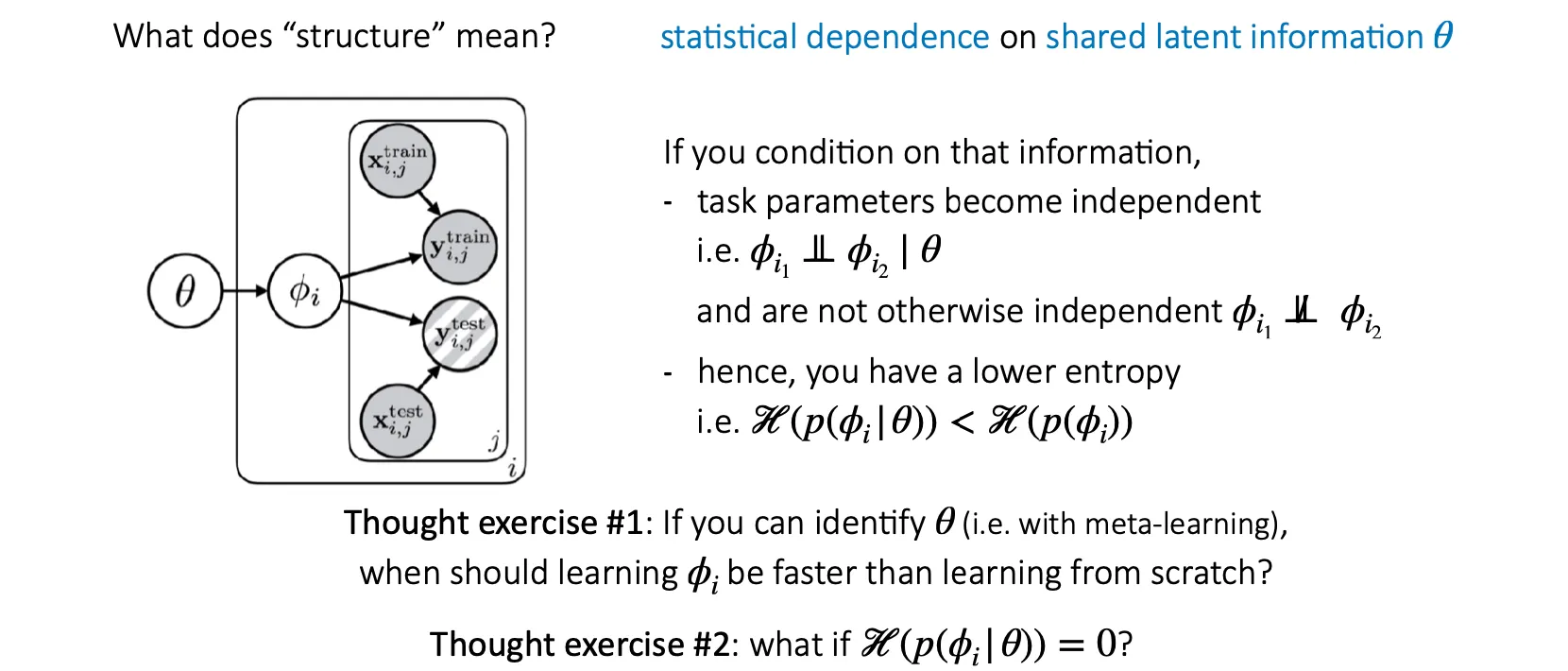
Task-specific parameter 는 에 의존하고 있고, 각 들은 given 에서 독립이다.즉, 이 경우에는 가 보다 작다.
#1 가 보다 매우 작을 경우, learning from scratch 보다 로부터 에 대한 힌트를 얻는게 더 학습이 빨리 될 것이다.
#2 일 경우는 자체가 의 task를 푸는데 학습이 필요 없이 그대로 모두 잘 수행하는 경우이다.
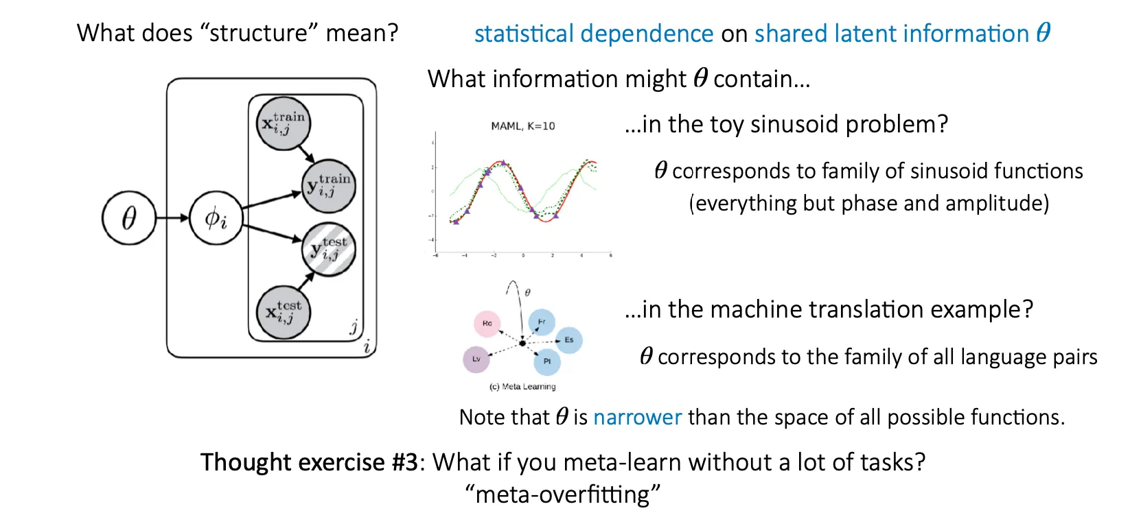
#3 Task가 많이 없이 meta-learning을 하면 어떻게 될까? Overfitting이 발생할 것이다.
Why be Bayesian?
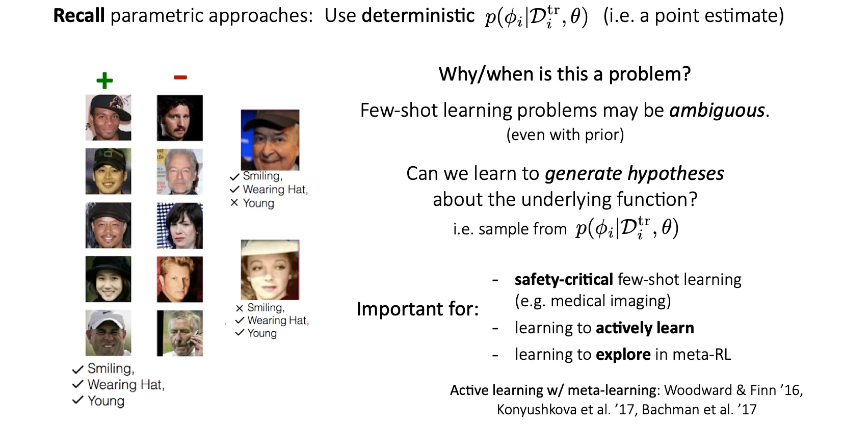
Parametric 접근방법에서, deterministic한 point estimate인 에서 나온 dataset을 사용하면, 그 양이 충분하지 않을 경우 task 자체가 ambiguous 해질 수 있다.
이때는, 에서 sampling을 해서 hypotheses를 생성해내는 아이디어를 생각해볼 수 있다.
이 상황은 safety가 중요한 분야나 active learning(부족한 부분은 알아서 더 학습하는), meta-RL에서 탐색하는 부분에서 중요하다.
Bayesian Meta-Learning Approaches
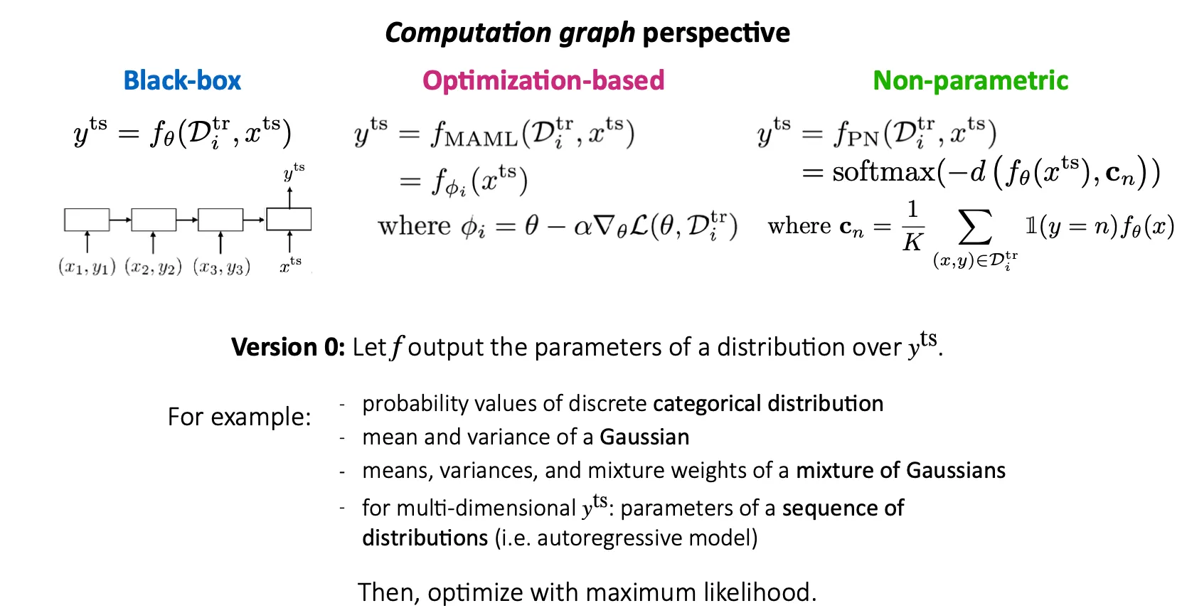
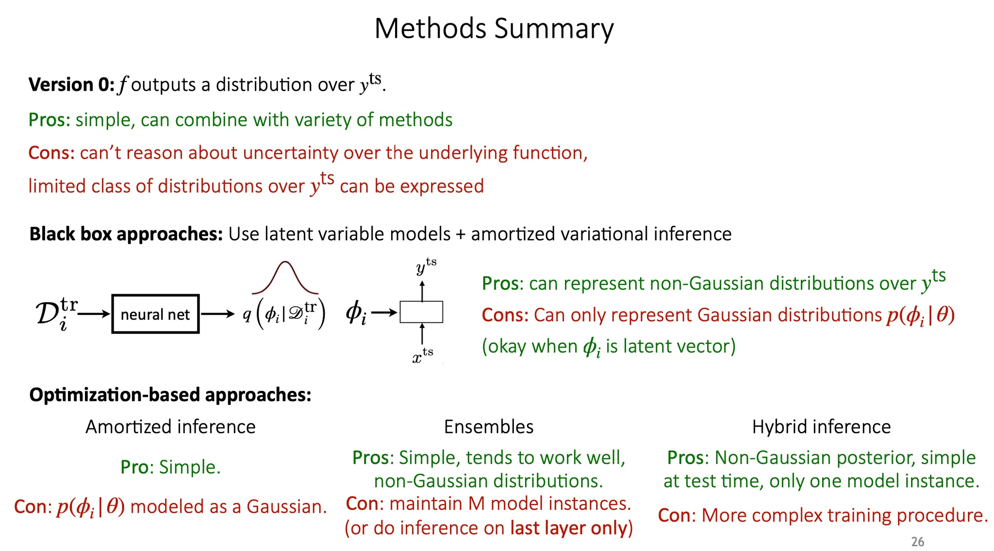
가장 단순한 방법으로는 의 분포에 대해 어떤 함수 가 그 분포의 parameter를 내놓도록 학습할 수 있다.
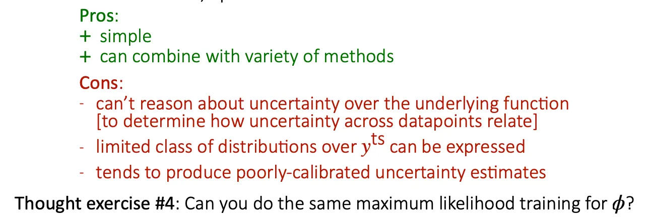
간편하고 쉽게 적용할 수 있지만, uncertainty를 분해해서 파악할 수 없다(모델 자체의 uncertainty인지, label noise인지 등). 또 가 표현될 수 있는 특정 형태의 분포에만 적용할 수 있다.
#4 이렇게 되면 를 학습할 때 maximum likelihood training을 그대로 적용하면 될까? ... 모르겠음ㅠㅠ
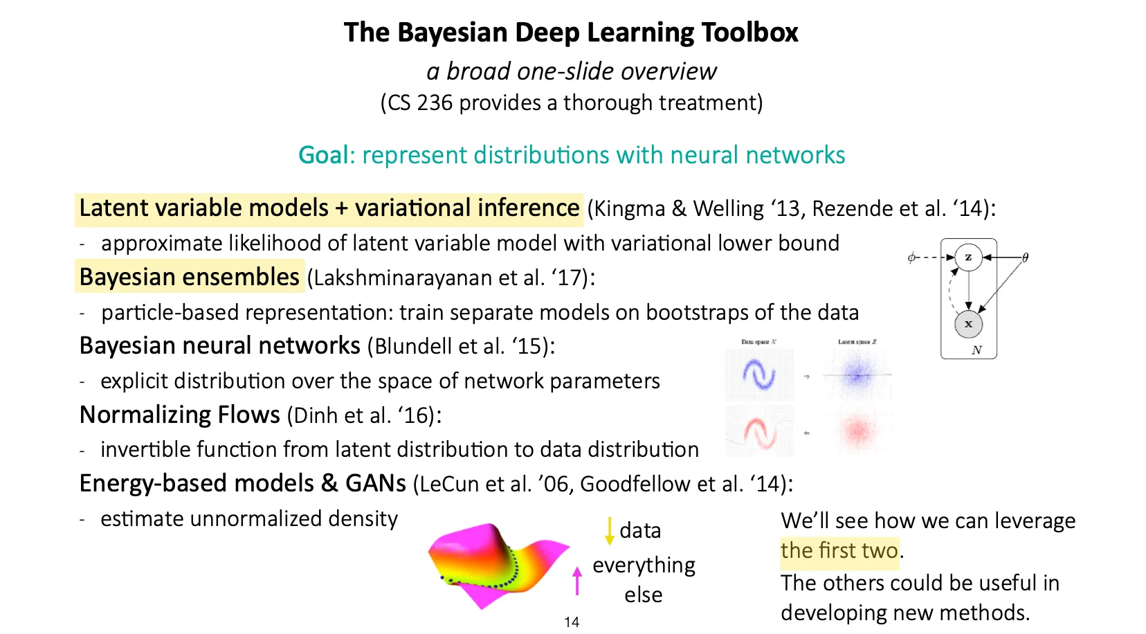
Deep learning에 Bayesian을 적용한 경우를 봐보자. 특히 latent variable model과 variational inference를 이용한 방법, Bayesian ensemble을 이용한 방법이 meta learning에 적용된 케이스가 있다. 2019년 기준으로 아래 세 개는 아직 적용 안 됨.
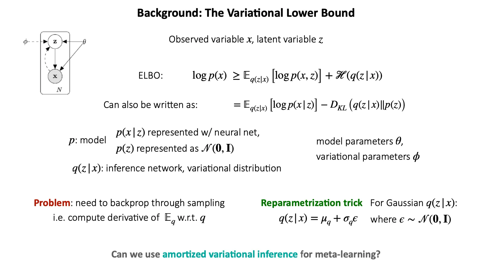
여기서 가 observed variable, 는 latent variable.
참고) Variational autoencoder에서는 는 decoder의 reconstruction loss이고, 은 inference network와 prior 사이의 KL divergence이다.
는 model이고, 는 neural net으로 표현할 수 있고, 는 학습된 mean과 variance로 표현할 수도 있다(VAE에서는 layer 이후에 mean과 variance가 등장하기 때문에 학습 안 된다).
는 inference network 또는 variational distribution을 의미한다.
여기서 문제는 sampling 은 differentiable 하지 않다는 것이다. 따라서, backpropagation을 위해 reparametrization trick을 사용한다.
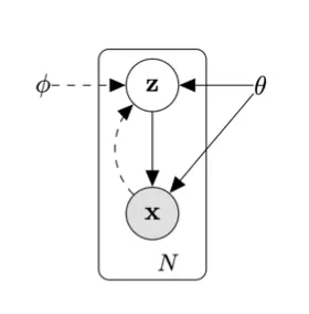
여기서 실선 화살표는 model distribution, 점선 화살표는 variational distribution 이다.
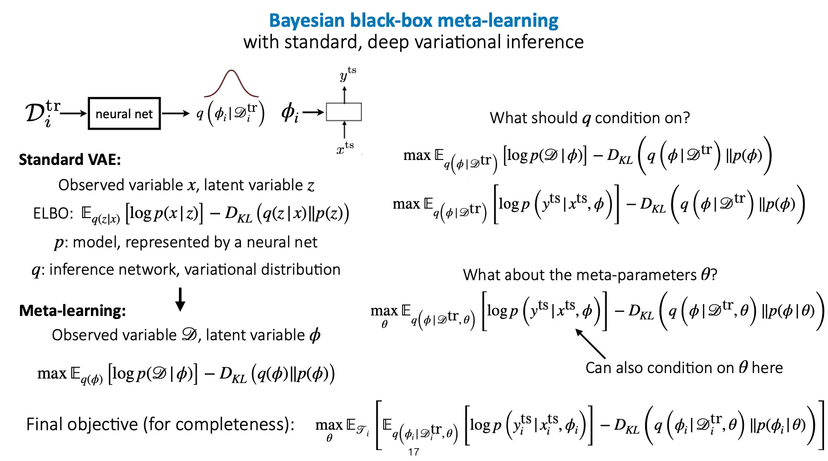
먼저 black-box meta-learning 부터 보면, 일반적인 VAE와 다르게 meta-learning에서는 observed variable을 data, latent variable을 (task-specific parameter)로 두고 학습을 진행하면 된다. 이 때 는 training data, 즉 에 condition을 두고 학습을 진행한다.
Meta parameter 역시 의 condition term으로 추가될 수 있다.
따라서, 최종 objective function은
이 된다. 이 때, 앞부분은 기존 meta learning(Bayesian이 없는)에서 최대화하고자 하는 바로 그 목적함수가 되고, KL divergence term은 q가 어떤 prior distribution에 가까워지도록 하는 부분에 해당한다.
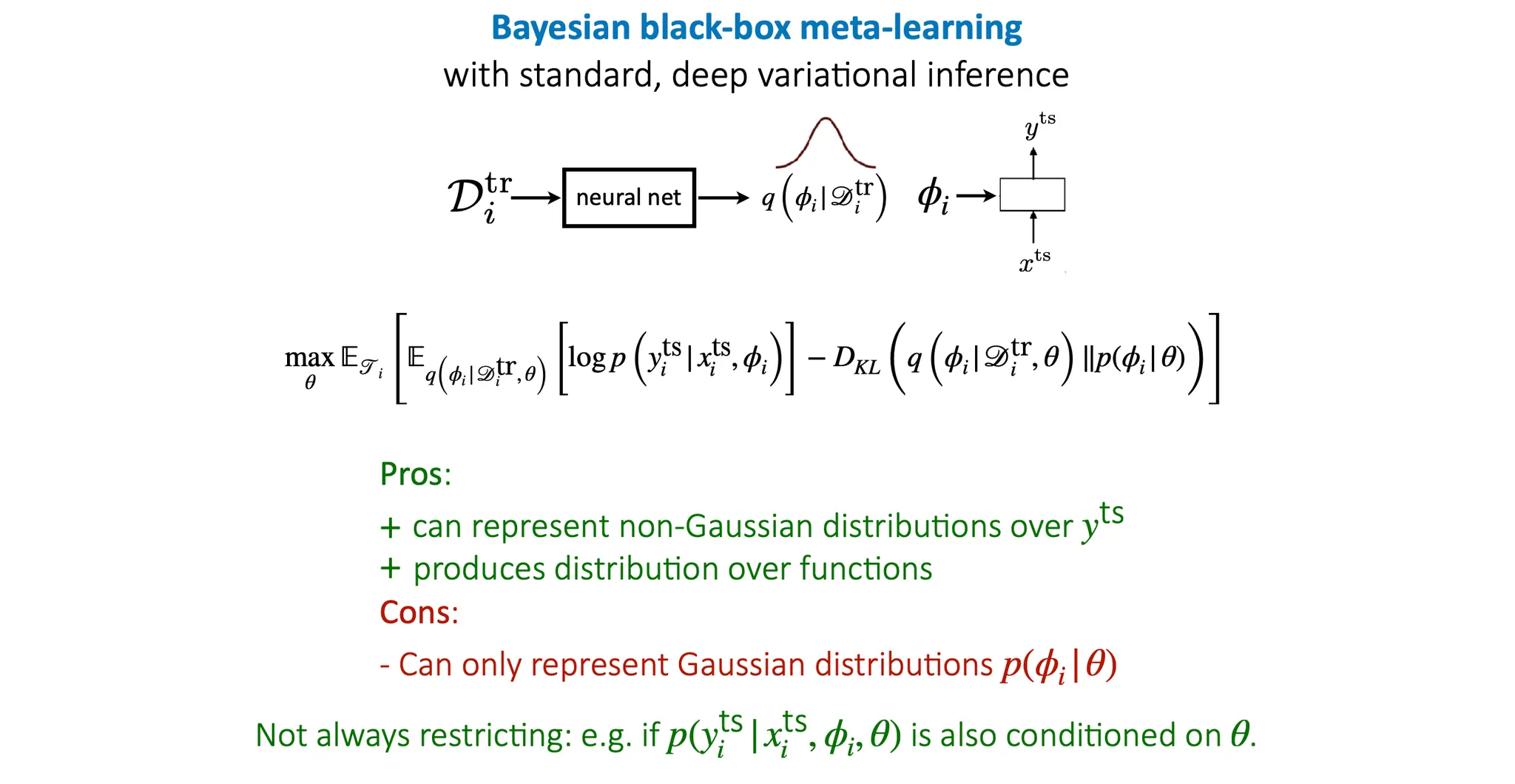
장점은..
•
에 대해서는 non-Gaussian 분포도 표현 가능
•
label의 distribution 뿐만 아니라 에 대한 distribution도 얻을 수 있음 → uncertainty 반영 가능
단점은..
•
는 Gaussian distribution만 가능
◦
Reparametrization trick을 Gaussian 형태로 쓰기 때문
◦
또, KL term이 non-Gaussian의 경우에는 closed-form으로 풀 수 없음
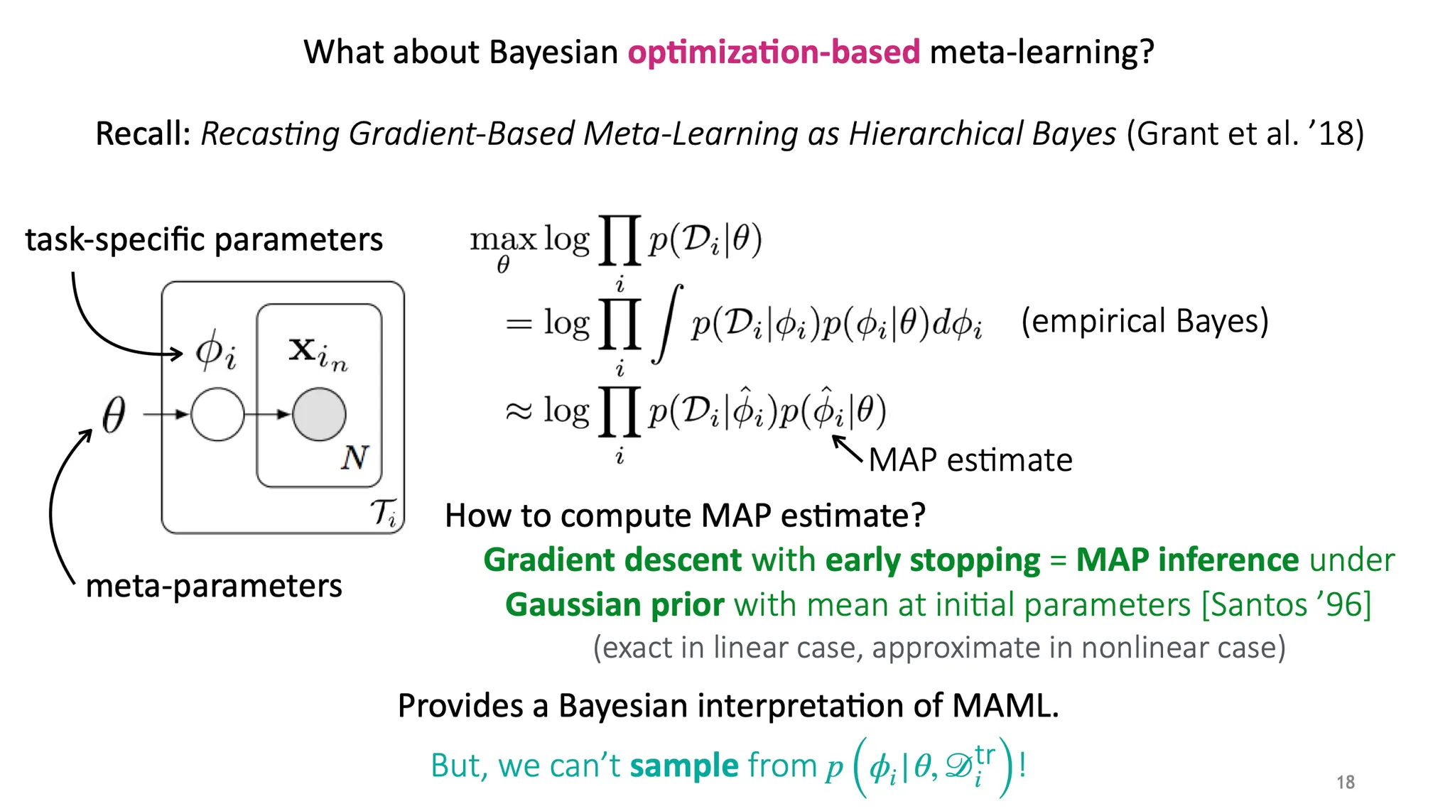
이전에 "Recasting gradient-based meta-learning as hierarchical Bayes" 라는 논문에서 MAML을 Bayesian 적으로 해석한 부분이 있었다. 하지만 하나의 MAP estimate를 사용하는 것은 하나의 parameter set만을 결정하는 것으로, 이는 에서 sampling을 할 수 없어서 우리가 원하던 Bayesian style이 아니다. 그럼 어떻게 해야될까?
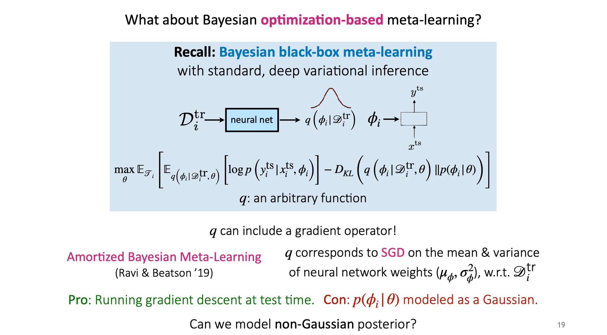
Black-box 방법에서 Bayesian을 적용했던 것을 다시 생각해보면, 는 어떤 함수든지 될 수 있었다. 이 는 꼭 neural network이 아니어도 되고, 의 분포를 표현할 수 있는 함수이면 된다. 이 가 gradient operator를 포함하는 형태이면 어떨까?
“Amortized Bayesian Meta-learning” 논문에서는 를 training data 학습 시 사용되는 neural network weight들의 mean 과 variance에 SGD를 가하는 것으로 적용했다.
장점은 간단히 test time 시에 gradient descent를 하여 meta parameter 를 update 할 수 있다는 점이다.
단점은 가 Gaussian으로 modeling 되어야 한다는 점인데, 그 이유는 앞에서 설명했듯이 backpropagate를 위해 reparametrization 할 때 Gaussian을 적용하고, KL-term을 closed form으로 만들기 위함이다.
그럼 posterior는 non-Gaussian으로 modeling 할 수 있을까?
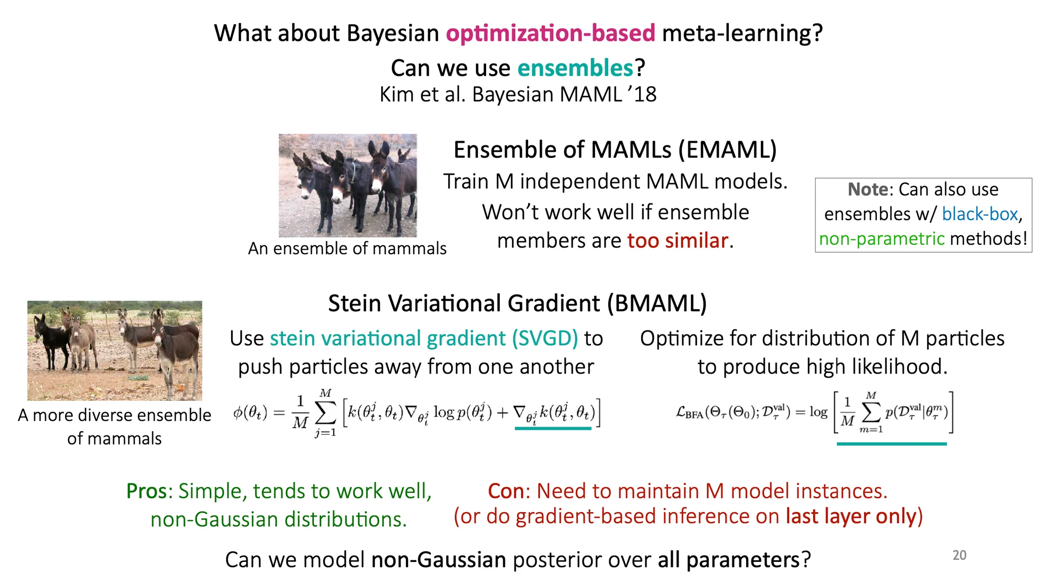
Ensemble을 활용하면 posterior를 non-Gaussian으로 모델링 가능하다.
그럼 모든 model instance를 보유하지 않고도 모든 parameter에 대해 non-Gaussian posterior를 모델링 할 수 있을까?
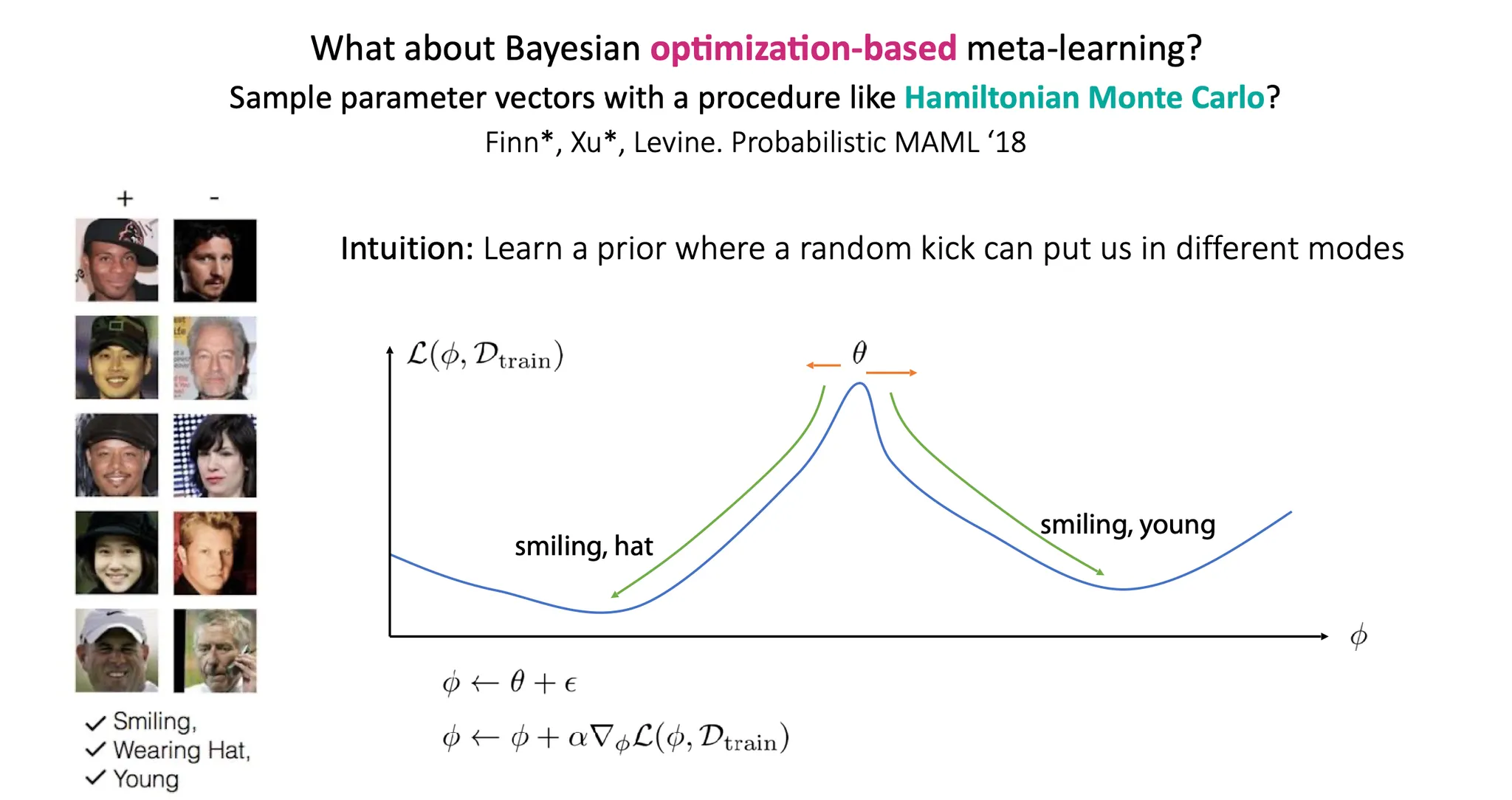
Hamiltonian Monte Carlo를 사용해 parameter vector를 sampling 하면 어떨까?
Probabilistic MAML은 어떤 random kick에 따라 다른 mode로 task-specific parameter 가 만들어질 수 있다는 intuition 하에 연구가 시작되었다.
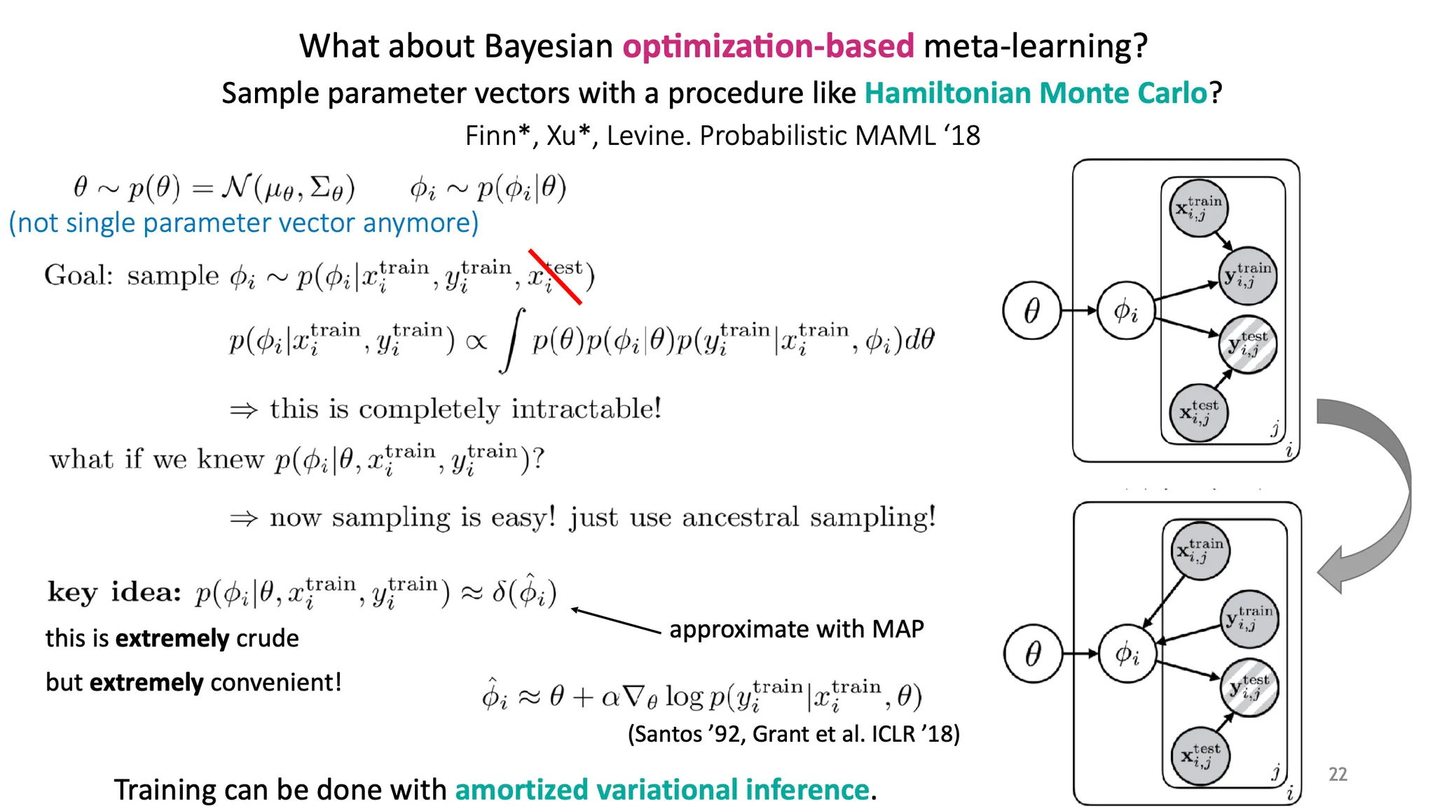
여기서 는 더 이상 하나의 고정된 parameter vector가 아니라 어떤 distribution 이다.
목적은 를 에서 sampling 하는 것이다. 이 때, 가 주어지지 않으면 는 independent 하므로 생략 가능하다(즉, 는 를 결정하는데 어떤 정보를 주지 않는다).
이 때, 은 intractable 해서 풀기 어렵다. 만약 우리가 를 알고 있다면? 그냥 parent node부터 sampling하는 ancestral sampling을 하면 되므로 훨씬 쉬워진다.
Crude estimate으로 를 ,즉, MAP로 estimate 하여 사용한다.
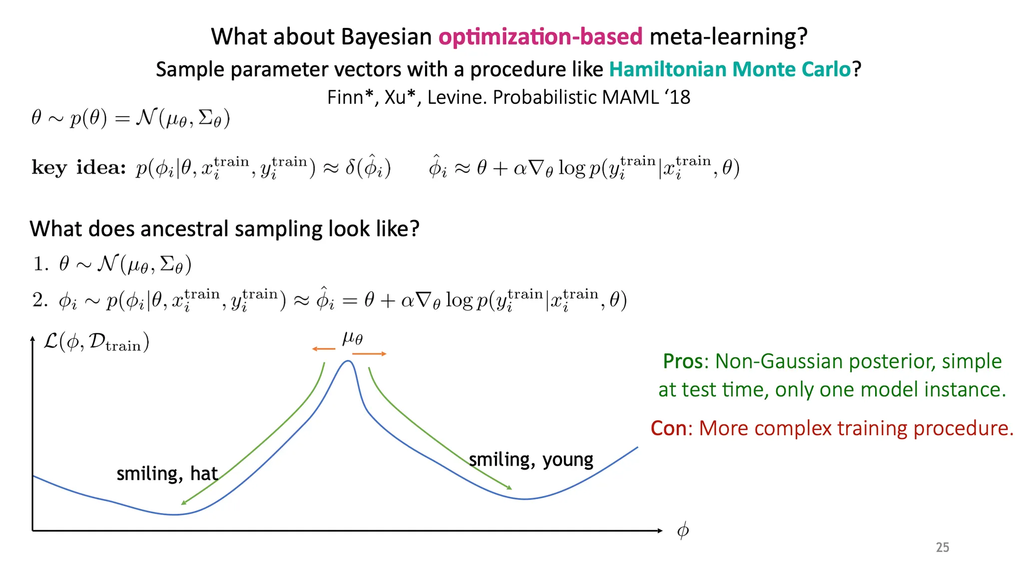
Ancestral sampling은 아래와 같이 진행된다.
1.
를 sampling 한다.
2.
는 에서 sampling하는데, 이 때 MAP estimate을 사용한다.
장점
•
Non-Gaussian posterior를 얻을 수 있고, 하나의 model instance만 가지고 있어도 된다.
단점
•
Crude estimate이다.
•
학습이 다소 복잡해질 수 있다.
How to evaluate Bayesian meta-learners?
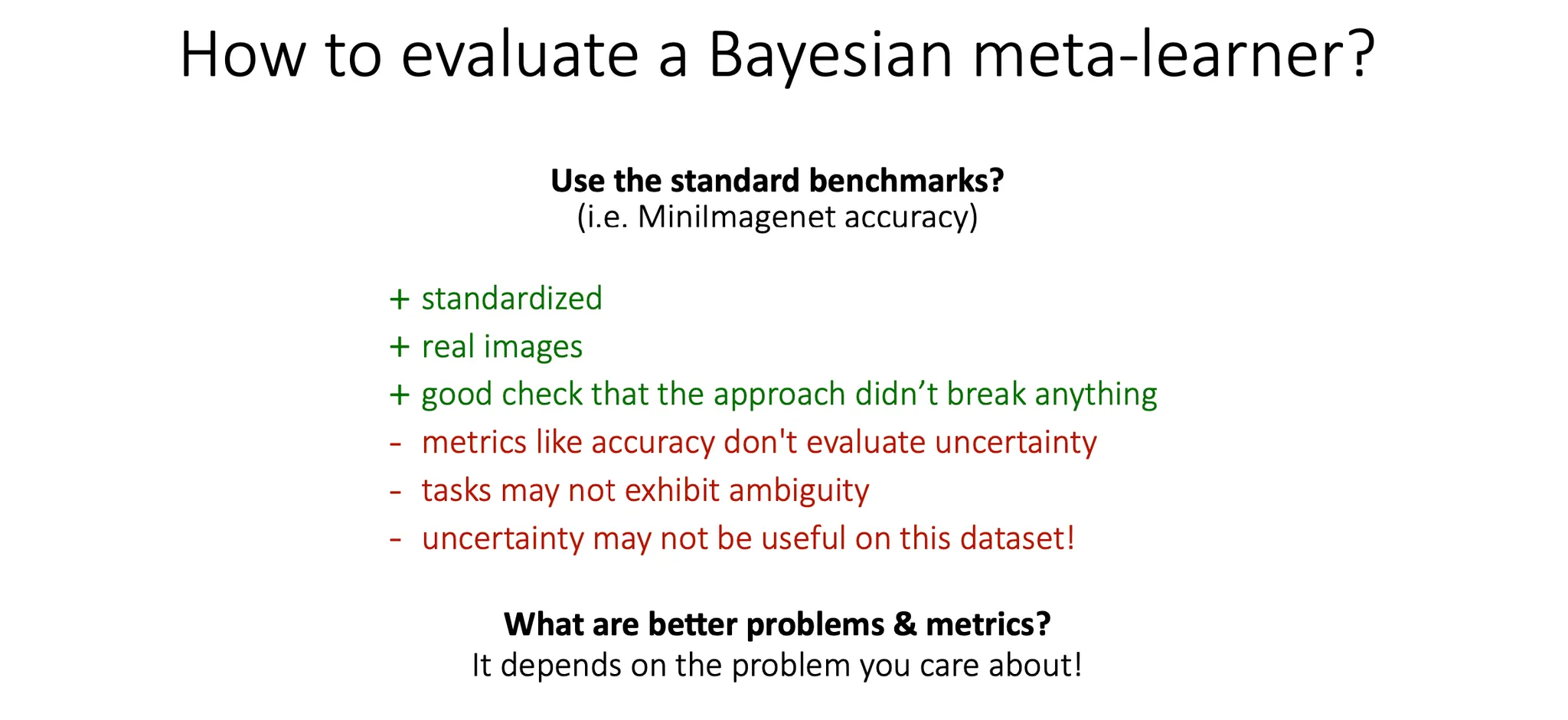
Bayesian meta learner 를 평가하는 방법은 무엇이 있을까?
Standard benchmark를 사용하면..
장점
•
표준화되어 있고, 실제 이미지이다.
•
이 방법의 적합성을 평가할 수 있다.
단점
•
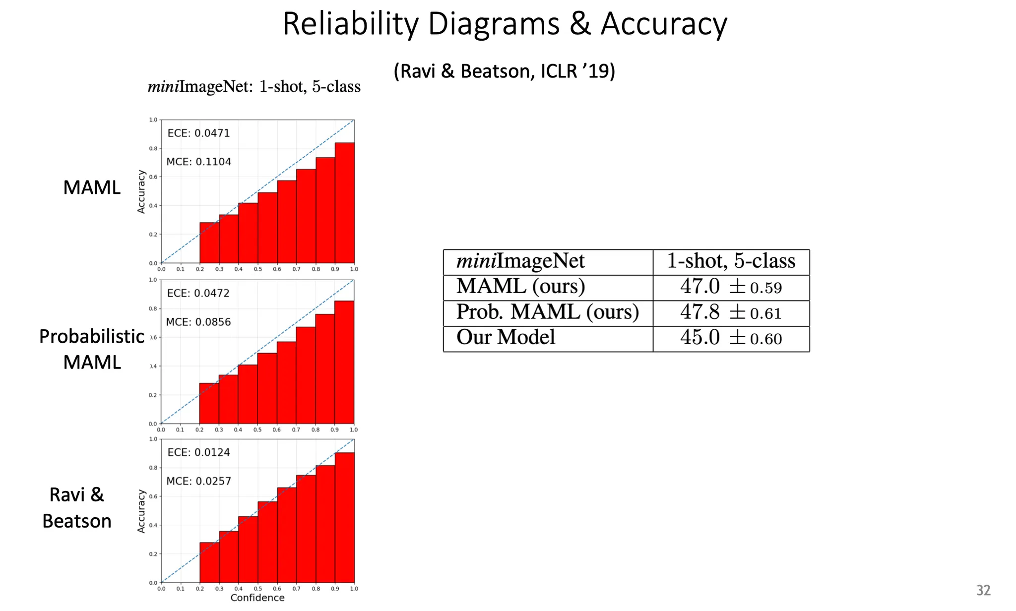
Accuracy까지는 당연히 측정할 수 있지만, uncertainty를 평가하기 어렵다.
•
Standard benchmark dataset이 ambiguity를 반영하지 못 하거나, uncertainty가 중요하지 않을 수 있다.
더 좋은 task나 평가 방법이 있을까? 그건 풀고자하는 문제에 따라 다르다.
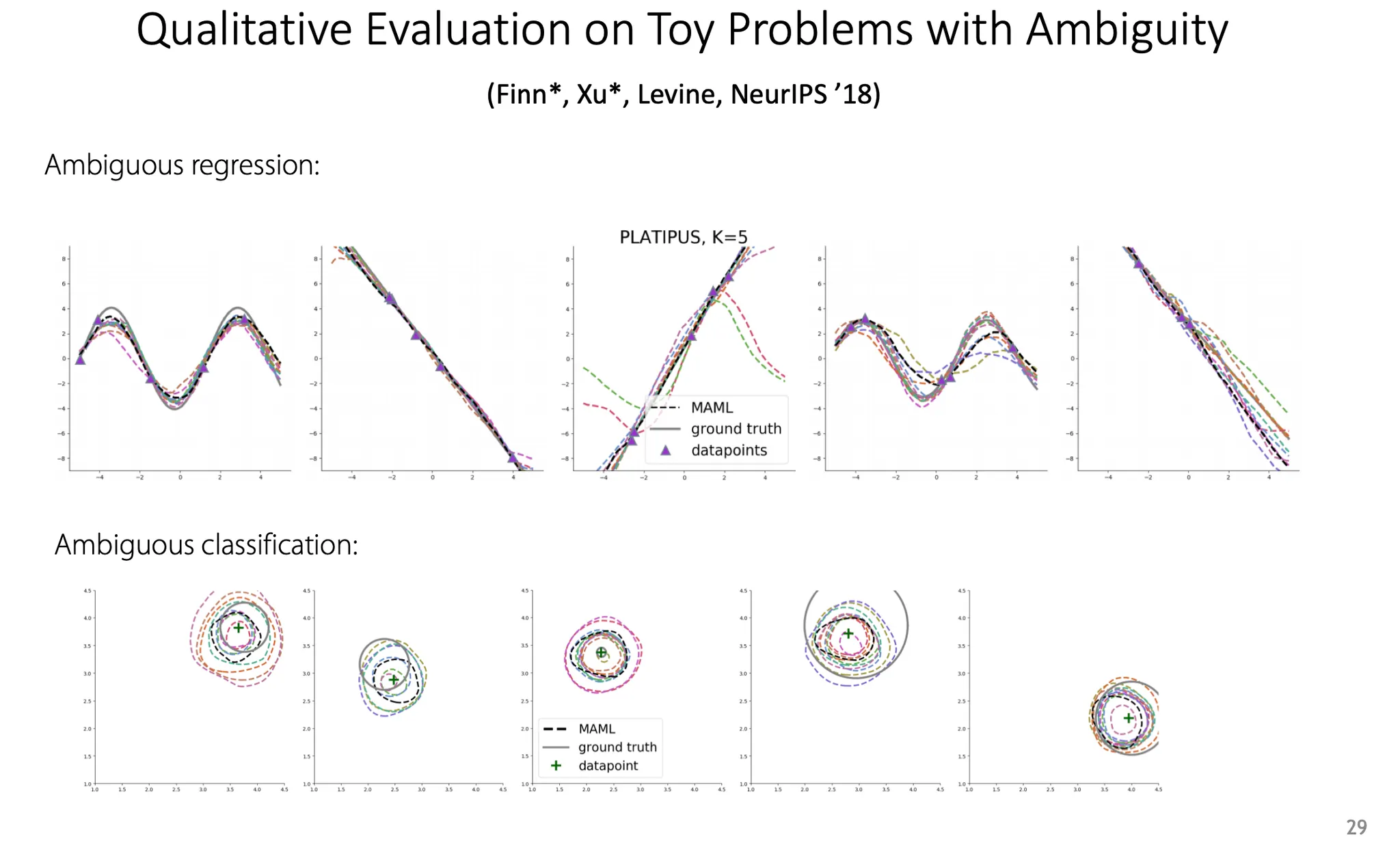
예를 들어, regression이나 classification task에서 ambiguity를 보기 위한 하나의 방법으로 위 그림과 같은 task를 학습하도록 할 수도 있다. 하지만 이건 real-world problem은 아니다.
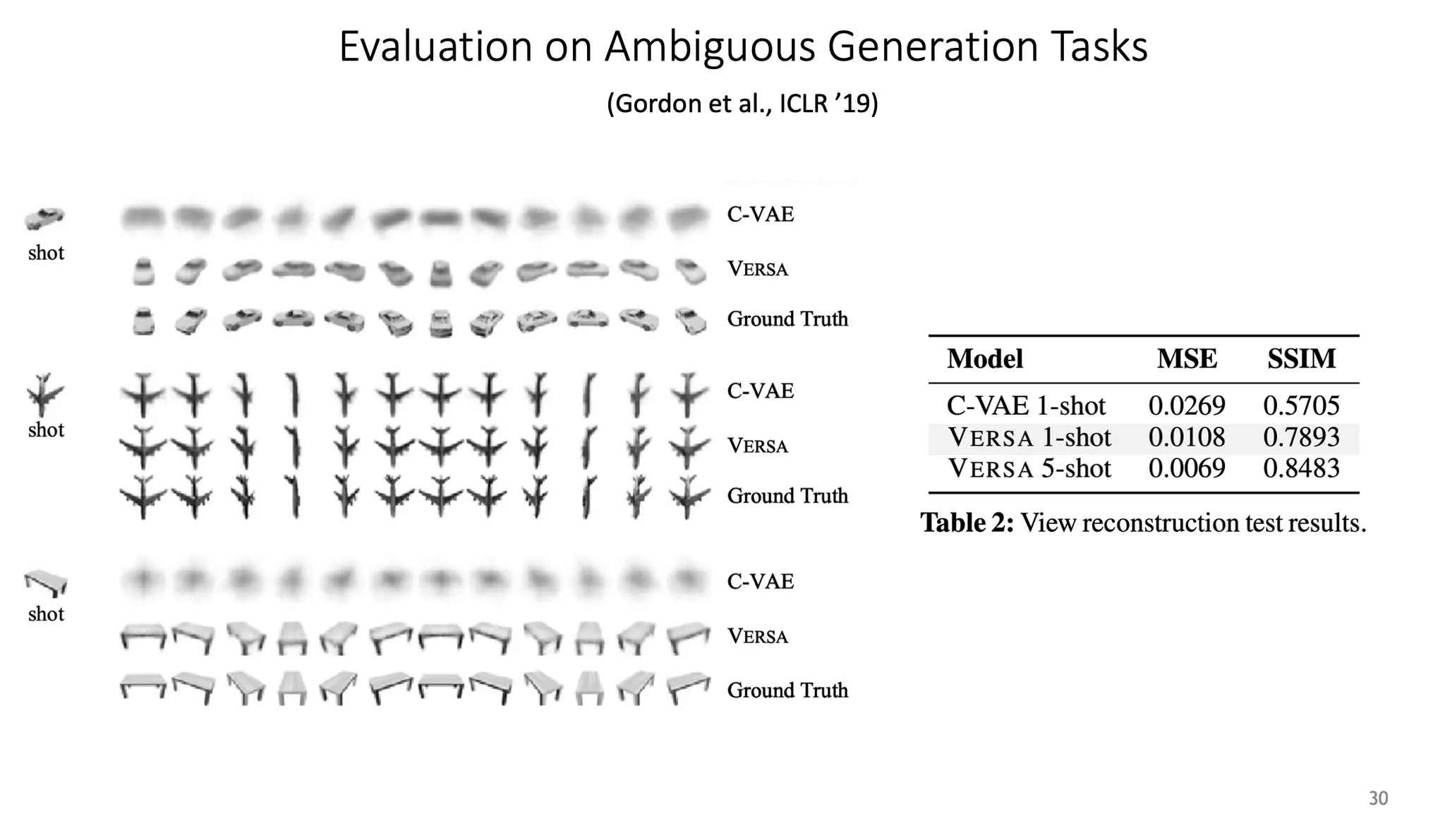
Generative model의 관점에서, one-shot learning 상황의 result이다. 이것은 ground truth와 비교하여 정량적으로 평가하였다.
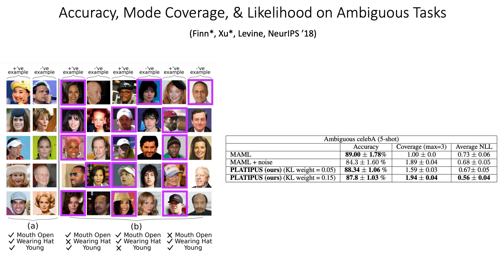
Accuracy, coverage, negative log likelihood 등 다양한 metric을 제공할 수도 있다.
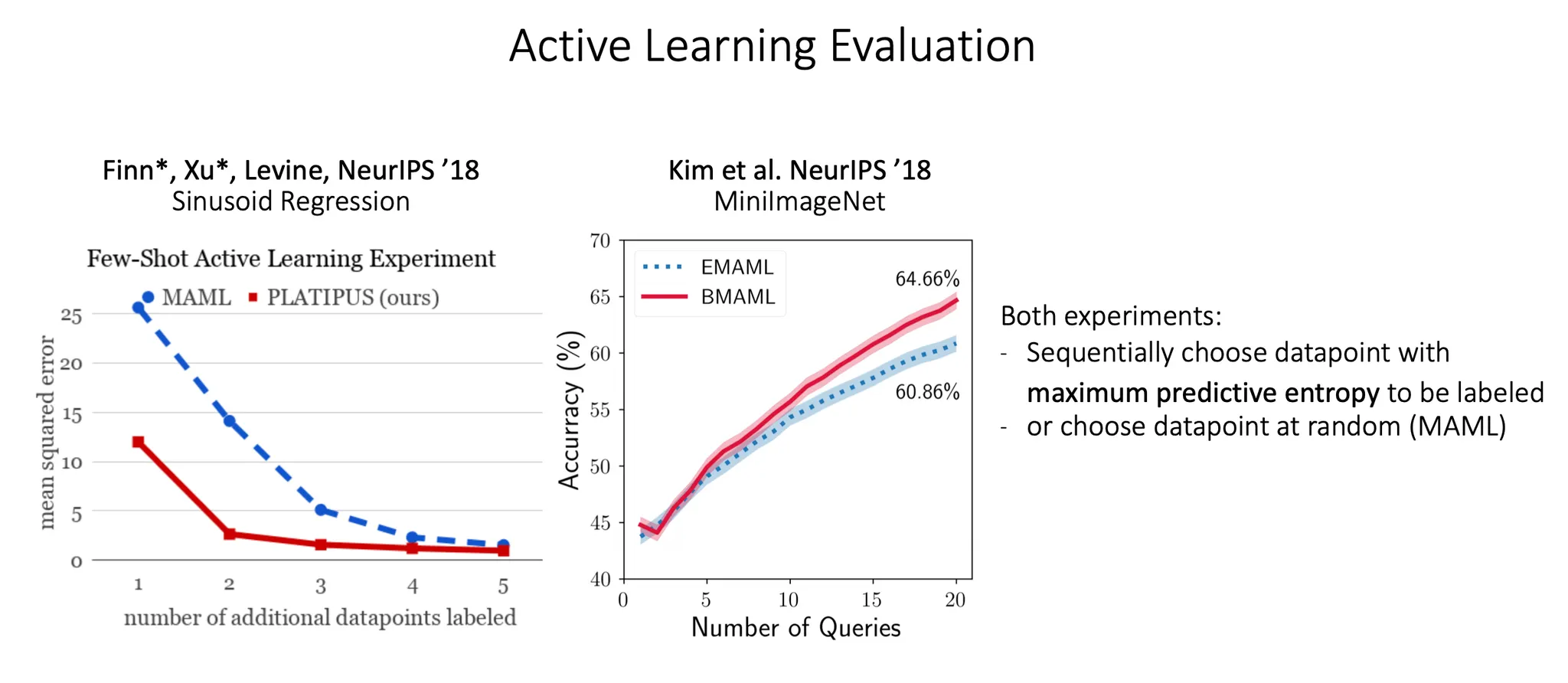
Active learning 관점에서 실험한 result. 어떤 datapoint를 봐야할지를 더 학습을 잘 할 수 있을지를 maximum predictive entropy 이용해서 선택한다.
이번 시간에는 uncertainty를 반영할 수 있는 meta learning에 대해 공부했다.