

Introduction
e3nn은 -equivariant neural network 의 약자로, 현재 (2023.09) PyTorch 및 Jax 기반의 Python package를 제공하고 있다.
먼저, 어떤 상황에서 equivariance 가 필요할까?
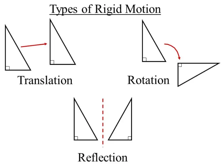
3차원 상에서 회전 (rotation), 이동 (translation), 반사 (reflection) 중 하나 이상에 대해 관계 없이, 같은 성질을 가져야 하는 상황을 생각해보자. 예를 들어, 어떤 분자 구조는 3차원 상에서 회전이나 이동을 한다고 해서 성질이 변하지 않는다 (반사의 경우 광학적인 성질이 변하는 경우도 있다). 이런 3차원 상의 좌표를 위 세 가지 rigid motion 중 하나 이상에 관계 없이 동일한 성질을 띄도록 모델링 해줄 수 있는 방법이 필요하다.
즉, 수식으로 표현하면, 모든 rigid motion 에 대해 를 만족해야 한다.
https://slideplayer.com/slide/9976677
3차원 상의 데이터도 neural network로 다루는 경우가 빈번해지면서, neural network 자체가 E(3) equivariance를 띄도록 설계한 것 중의 하나가 e3nn 이다.
설치 및 공식 Tutorial은 아래 링크를 참고하자.
이 포스팅에서는 e3nn package에서 가장 많이 쓰는 module인 e3nn.o3 에 대해 주로 다뤄본다.
이를 이해하는데 있어 중요한 기초 지식은 아래 페이지를 참고!
Orthogonal group
•
: Orthogonal group in 3D. Group of 3D orthogonal matrices.
즉, 를 만족하는 matrix의 group을 의미한다.
는 rotation (회전)과 inversion (reflection, 거울반사)으로 구분할 수 있다.
Rotation group은 “Special Orthogonal group ” 라고도 불리고, 정의에 따라 이다. 이들은 스스로 group 을 이룬다.
Inversion은 이다. 이들은 스스로 group을 이루지 못 한다. Inversion matrix 두 개를 곱하면 인 matrix 가 나오기 때문이다.
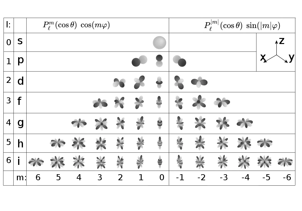
Spherical harmonics
•
Sphere의 surface에서 정의된 special function 이다.
•
의 irreducible representation의 basis function 이다.
e3nn.o3
1. Irreps (irreducible representations)
from e3nn.o3 import Irreps
# example
irreps = Irreps("1o") # (count=1이 생략되어 있음), degree=1, parity=odd. 1x1o 로도 표현.
mul_ir = irreps[0]
mul, ir = mul_ir # count, (degree, parity)
l, p = ir # degree, parity
Python
복사
참고) Parity
2. TensorProduct
모든 tensor product는 로 표시하고, 아래 두 특징을 가진다.
1.
Bilinear:
•
•
2.
Equivariant
•
이 때 는 의 symmetry operation.
TensorProduct operation 를 수행할 때, 그 결과값의 irreps type은 와 의 irreps type에 의해 결정되고, 여러 path가 있을 수 있다. 이는 아래와 같이 정의된다.
다시 말해,
•
Output degree 은 두 input degree간의 차와 합 사이의 개수 () 만큼의 경우가 가능하다.
•
Output parity 는 두 input parity를 곱해서 결정된다. Parity는 -1 (odd) 또는 1 (even)의 값을 가지므로, 아래 표처럼 계산된다.
(-1) | (-1) | (1) |
(-1) | (1) | (-1) |
(1) | (-1) | (-1) |
(1) | (1) | (1) |
TensorProduct 계산 예시
e3nn.o3.TensorProduct class가 다양한 operation을 지원하지만, 그 하위 subclass마다 주된 사용처가 구분되어 있다. 따라서 주로 subclass (FullTensorProduct, FullyConnectedTensorProduct, ElementwiseTensorProduct, TensorSquare)를 사용하게 된다.
•
FullTensorProduct
from e3nn import o3
# example
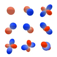
tp = o3.FullTensorProduct(
irreps_in1='2x0e + 3x1o',
irreps_in2='5x0e + 7x1e'
)
tp.visualize()
Python
복사
FullTensorProduct는 가장 기본적인 연산이라고 생각하면 된다.
두 input irreps의 모든 pair에 해당하는 output irrep을 return 한다.
count x (irreps type) | count x (irreps type) | count x (irreps type) |
, , | ||
•
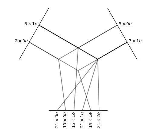
FullyConnectedTensorProduct
# example
tp = o3.FullyConnectedTensorProduct(
irreps_in1='5x0e + 5x1e',
irreps_in2='6x0e + 4x1e',
irreps_out='15x0e + 3x1e'
)
tp.visualize();
Python
복사
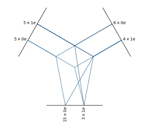
선이 회색이 아니라 파란색인 이유는 이들이 learnable 하기 때문이다.
FulllyConnectedTensorProduct는 모든 path 중에서 irreps_out 에 해당하는 irreps만 return 하고, 각 output은 compatible path의 learned weighted sum이다. 이게 무슨 뜻일까?
count x (irreps type) | count x (irreps type) | count x (irreps type) |
먼저, 앞에 있는 숫자보다 irreps의 type ( 등)에만 집중해보자. Input irreps에 해당하는 irreps type은 뿐이다. 이때, 를 얻는 경우의 수가 가지가 있지만, output irreps 중 에 해당하는 것은 15개만 return 하면 된다. 즉, 15개의 각 element를 얻을 때 50개의 숫자를 learnable parameter에 의해 weighted combination 해서 얻는다.
참고로, 모든 가능한 output irreps type이 irreps_out에 명시되어야 하는 것은 아니다. 예를 들어보자.
# example
tp = o3.FullyConnectedTensorProduct(
irreps_in1='5x1o',
irreps_in2='3x1o',
irreps_out='20x0e')
tp.visualize()
Python
복사
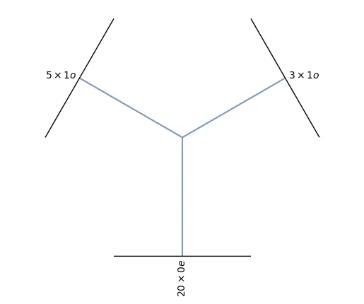
위의 경우, 원래 output irreps type으로 가 가능하지만 그 중 에 해당하는 것만 return 한다. 이때도 20개의 type output element는 15개의 type input element들을 learnable parameter에 의해 weighted combination 해서 얻는다.
•
ElementwiseTensorProduct
# example
tp = o3.ElementwiseTensorProduct(
irreps_in1='5x0e + 5x1e',
irreps_in2='4x0e + 6x1e')
tp.visualize()
Python
복사
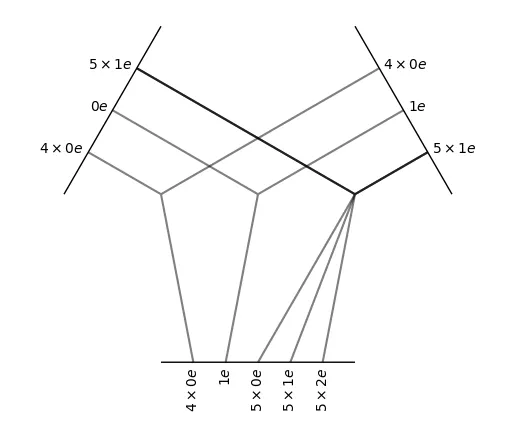
Elementwise tensor product에서는 각 irrep type끼리 one-by-one 으로 곱해진다.
Type이 맞는 것들끼리만 먼저 계산하고, count가 남으면 그들은 따로 분리되어 계산된다.
•
TensorSquare
# example
tp = o3.TensorSquare("5x1e + 2e")
tp.visualize()
Python
복사
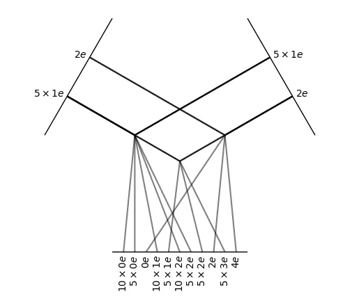
스스로의 non-zero entity 간의 tensor product operation을 수행한다.
이 operation은 다른 operation과 normalization이 다르게 적용된다고 한다.
3. spherical_harmonics
Spherical harmonics 는 unit sphere (구면체)에서 정의된 함수이고, sphere 에서의 basis를 형성한다.
e3nn.o3.spherical_harmonics(
l: int | List[int] | str | Irreps,
x: Tensor,
normalize: bool,
normalization: str=’integral’)
Python
복사
3차원 공간에서 정의된 polynomial 이다.
이때, normalize=True 를 하게 되면
아래 조건을 만족한다.
•
Cartesian coordinate x, y, z의 polynomial 이다.
•
Equivariant 하다:
•
Orthogonal 하다:
◦
Constant value는 normalization choice에 따라 달라진다.
Parameters:
•
l (int or list of int): spherical harmonics의 degree
•
x (torch.Tensor): tensor of shape (…, 3)
•
normalize (bool): input x를 normalize 해서 unit vector로 만들어 sphere에 있도록 할 것인지 (spherical harmonics에 projection 하기 전에)
•
normalization ({’component’, ‘norm’, ‘integral’}): output tensor를 어떻게 normalize 할 것인지.
◦
component:
◦
norm: . 즉, component / sqrt(2l+1)
◦
integral: . 즉, component / sqrt(4pi)
# example
a = torch.rand(10, 3)
sh = o3.spherical_harmonics(2, a, normalize=True, normalization="component")
print(a) # (10, 3)
print(sh) # (10, 2*2 + 1)
Python
복사
# output
tensor([[0.0339, 0.1357, 0.4650],
[0.4342, 0.7297, 0.7079],
[0.4223, 0.6162, 0.7941],
[0.4146, 0.9159, 0.1536],
[0.1951, 0.9450, 0.7876],
[0.9178, 0.5146, 0.5664],
[0.2060, 0.1604, 0.8237],
[0.6062, 0.2706, 0.6967],
[0.7771, 0.5898, 0.6000],
[0.5828, 0.9508, 0.0527]])
tensor([[ 0.2591, 0.0756, -0.8562, 1.0363, 1.7664],
[ 0.9742, 1.0041, 0.3432, 1.6370, 0.4953],
[ 1.0926, 0.8479, -0.0464, 1.5945, 0.7368],
[ 0.2384, 1.4218, 1.6022, 0.5268, -0.2776],
[ 0.3836, 0.4603, 0.8128, 1.8580, 0.7267],
[ 1.4099, 1.2809, -0.4961, 0.7905, -0.7073],
[ 0.8803, 0.1714, -1.0024, 0.6854, 1.6496],
[ 1.7662, 0.6861, -0.8528, 0.7885, 0.2464],
[ 1.3766, 1.3533, -0.2286, 1.0447, -0.3602],
[ 0.0954, 1.7218, 1.3146, 0.1557, -0.5234]])
Plain Text
복사