Recommender Systems
1. Task and Evaluation
•
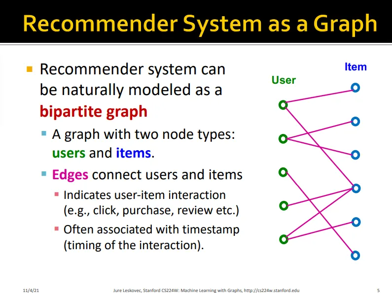
user와 item, 두 가지 노드로 이루어진 bipartite graph
•
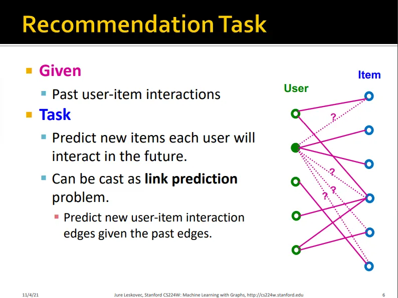
recommendation task란 과거의 user-item interaction을 통해 새로운 user-item interaction을 예측하는 link prediction으로 볼 수 있음
•
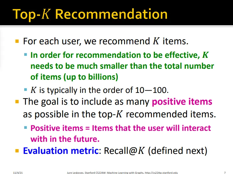
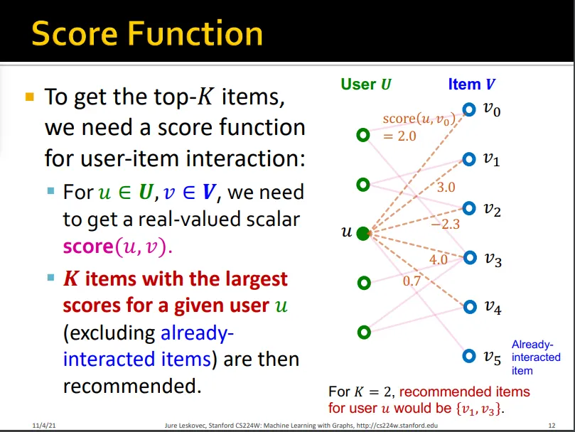
유저에게 K개의 item을 추천해주고 가장 interact할 가능성이 높을 item을 추천해주는게 목표
•
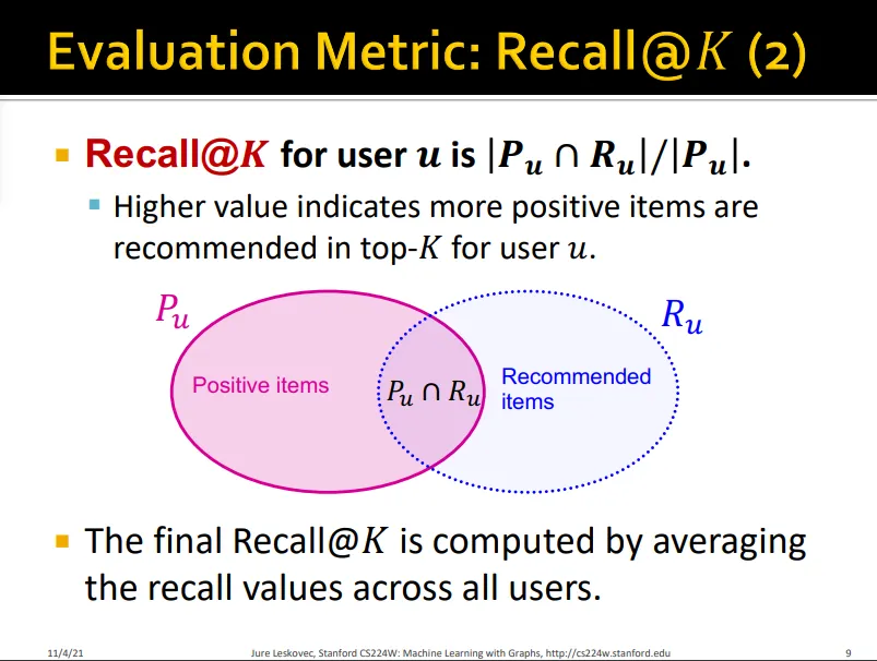
주로 Recall @K를 evaluation metric으로 사용
•
Recall@K는 K개의 item을 추천했을 때 해당 유저가 실제 고른 item에 대한 추천받은 item의 비
•
보통 전체 유저의 recall 값을 평균하여 계산
2. Embedding-Based Models
•
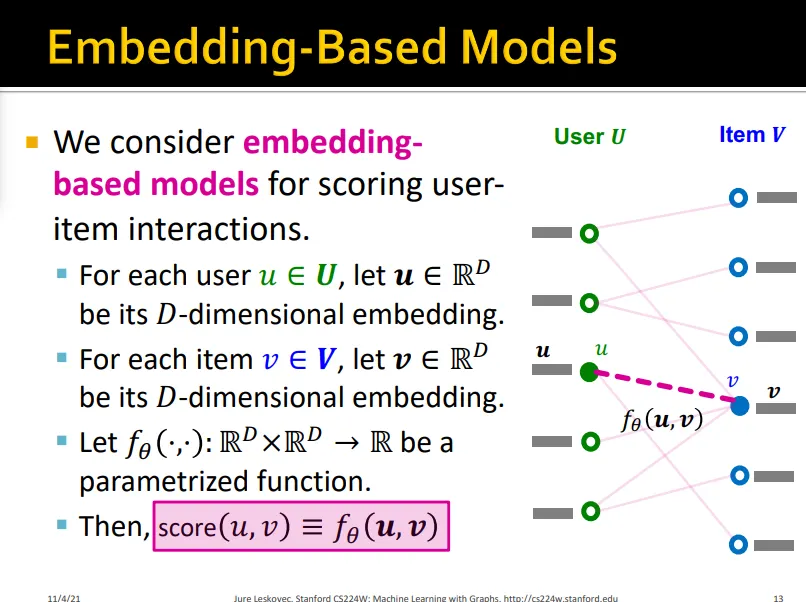
top-K개의 item을 고르기 위해 scalar score를 구할 필요가 있음
•
user와 item의 embedding을 이용해 scoring을 하고자 함
•
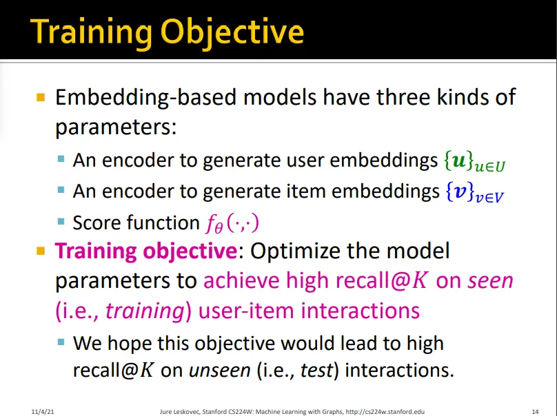
user/item embedding을 위한 encoder와 score function이 seen user-item interaction에서 high recall@K를 내도록 학습
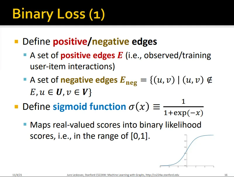
2.1. Surrogate Loss Functions: Binary Loss
•
positive/negative edge prediction
•
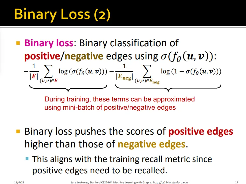
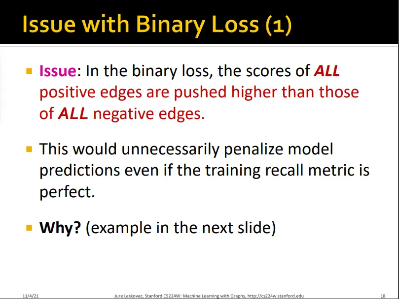
Binary loss는 positive edge의 score가 negative보다 더 높아지도록 함 (binary loss는 edge가 positive인지 negative인지가 중요하므로)
•
하지만 binary loss는 모든 positive edge를 모든 negative edge보다 높은 score를 갖게 하는 데에만 초점을 둠
•
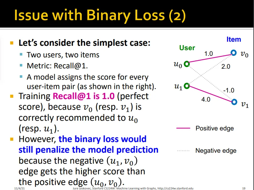
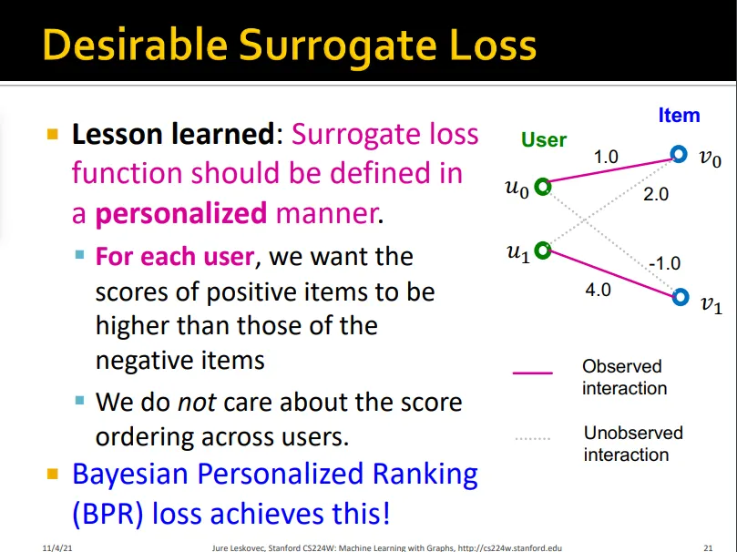
예를 들어, 아래 모델은 positive edge prediction을 잘했음에도 불구하고, 2.0의 score를 갖는 negative edge가 1.0의 score를 갖는 positive edge보다 score가 높기 때문에 모델은 계속해서 이를 penalize함
•
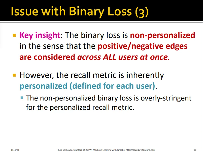
즉, binary loss는 user별로 personalized되어 있지 않음
•
따라서, 각 유저마다 positive item이 negative item보다 더 높은 score를 갖게 해야 함
2.2. Loss function: BPR Loss
•
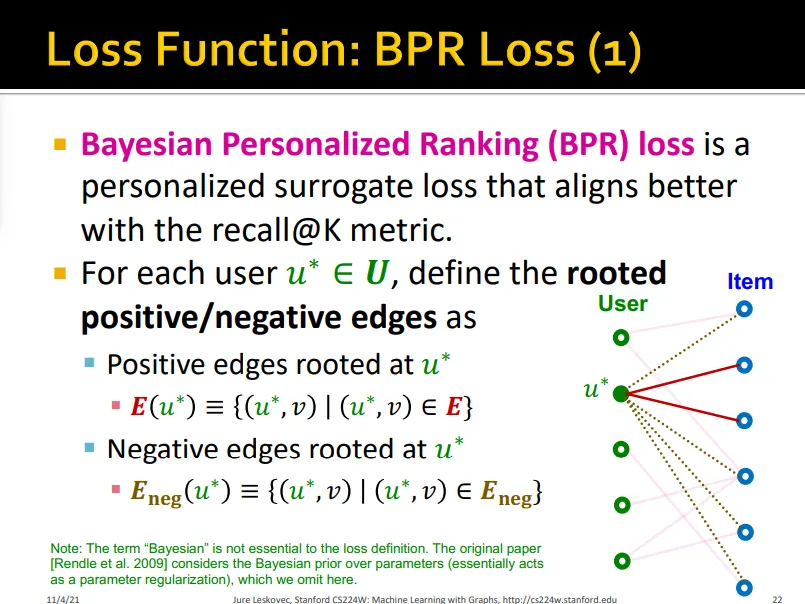
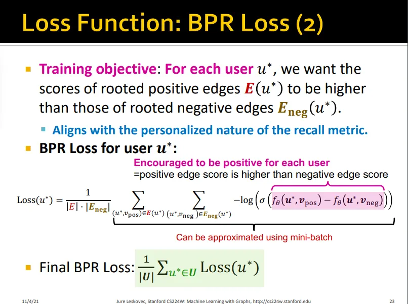
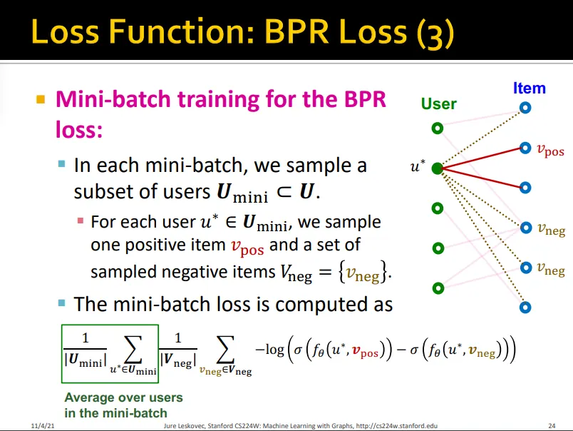
BPR loss는 user별로 positive/negative edge loss를 계산
•
user별로 positive edge의 score가 negative edge의 score보다 높아지도록 함
•
user별로 하나의 positive item의 score와 나머지 negative item의 score합의 차이
•
mini-batch 내 user set들에 대해 개별적으로 수행하여 loss average
•
Embedding model은 다른 비슷한 user들의 비슷한 선호를 반영하게 해줌
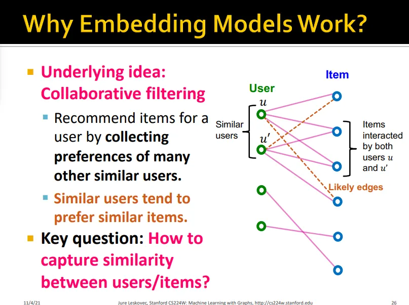
•
Embedding 모델은 user와 item 사이의 similarity를 잡을 수 있음
다음 장에선
→ Matrix factorization같은 conventional collaborative filtering에서 GNN으로 graph structure로 구현한 NGCF, LightGCN을 살펴봄
→ rich node attribute을 활용해 high-quality embedding을 만든 PinSAGE 모델을 살펴봄
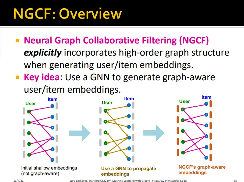
3. Neural Graph Collaborative Filtering
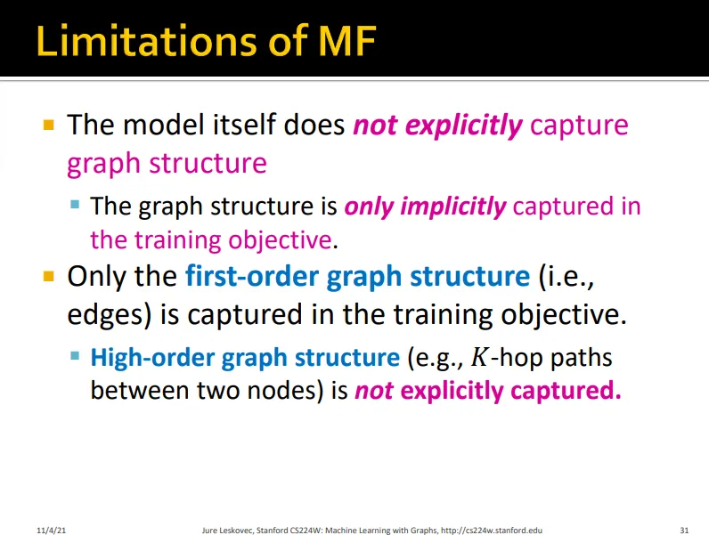
3.1. Conventional Collaborative Filtering
•
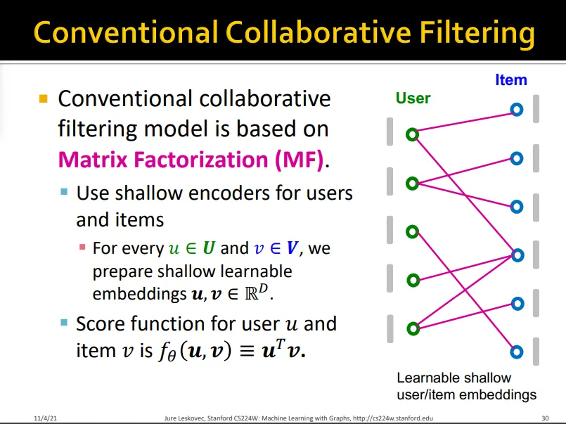
기존 CF는 matrix factorization을 바탕으로 함
•
그래프 구조를 잘 반영하지 못함
•
multi-hop에 있는 정보는 반영하지 못함
•
high-order 정보가 전파된 embedding을 만들겠다
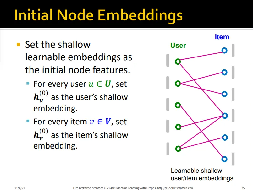
Step 1. Initial Node Embeddings
•
node feature로 initial node embedding
•
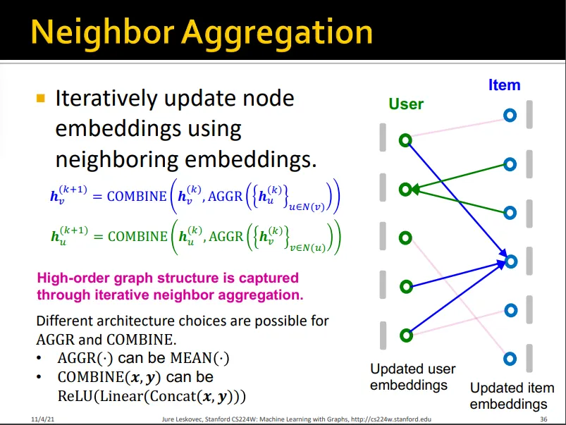
item은 연결된 user embedding을 aggregate해서 update
•
user는 연결된 item embedding을 aggregate해서 update
•
final embedding inner product하여 score구함
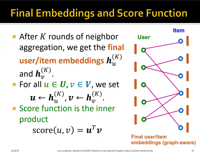
→NGCF는 conventional CF와는 다르게 high-order graph structure를 인지함
3.2. LightGCN
•
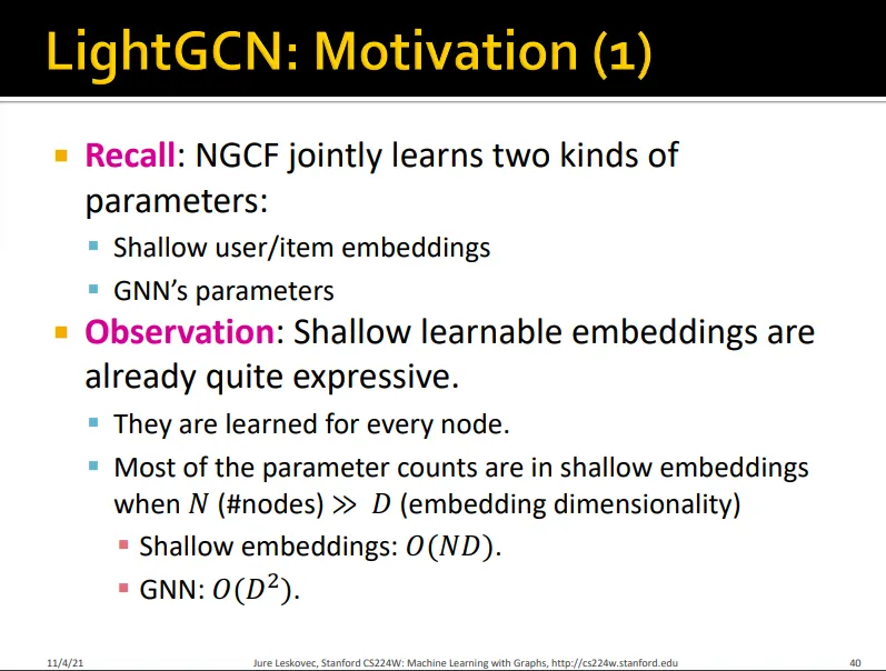
NGCF에서 학습하는 파라미터는 두 가지
◦
Shallow user/item embeddings
◦
GNN parameter
•
Shallow learnable embedding은 노드 단위로 이루어지기 때문에 충분히 expressive 함
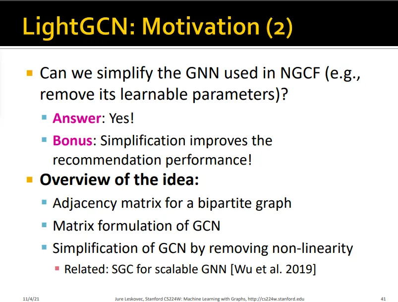
•
NGCF를 세 가지 방법으로 simplify함
•
recommendation performance가 더 향상되는 결과를 보임
•
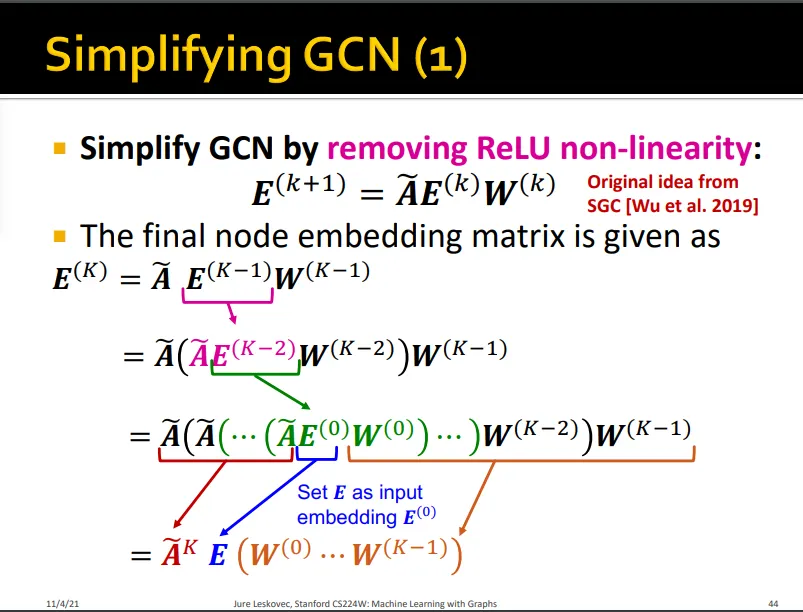
ReLU 제거
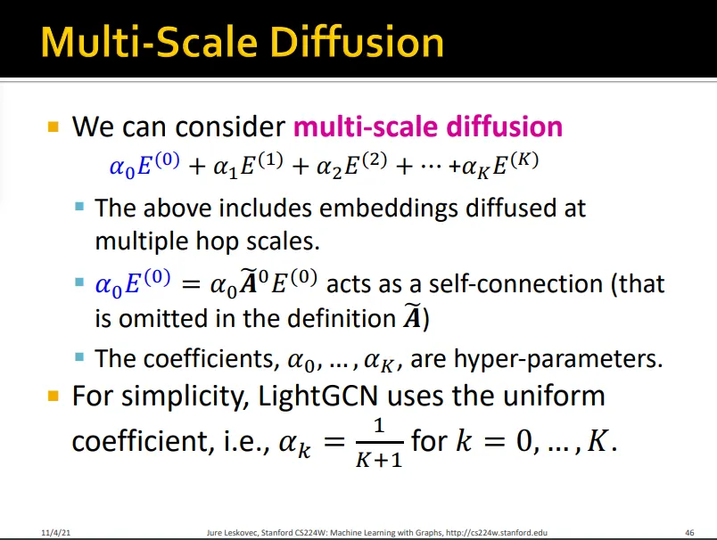
•
Smoothing되는 걸 방지하기 위해 각 layer의 에 가중치 를 곱해 더함
•
LightGCN에서는 uniform한 를 사용
•
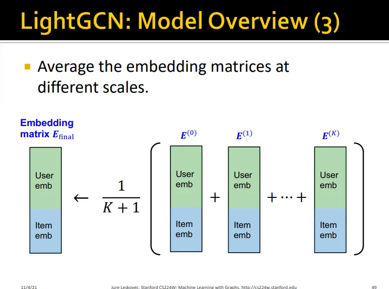
final embedding은 아래와 같음
•
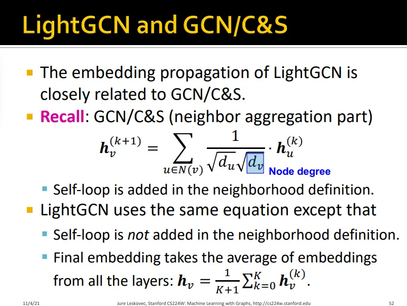
LightGCN이 GCN/C&S와 다른 점은
◦
Self-loop가 포함되지 않음
▪
multi-scale diffusion단계에서 self-loop 가 자연스럽게 들어갈 뿐
◦
Final embedding은 모든 layer embedding의 평균
•
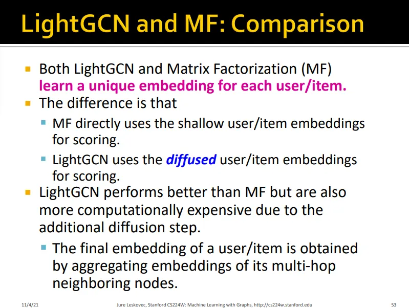
LightGCN이 MF와 다른 점은
◦
여러 층의 user/item embedding이 diffused되는 것
•
Shallow encoder만 학습된다는 점은 같음
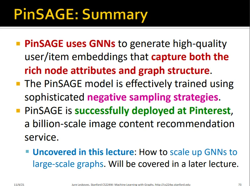
3.3. PinSAGE
•
negative sampling technique을 발전시킴
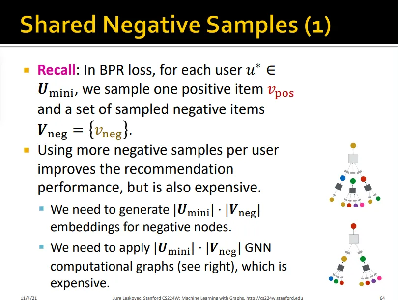
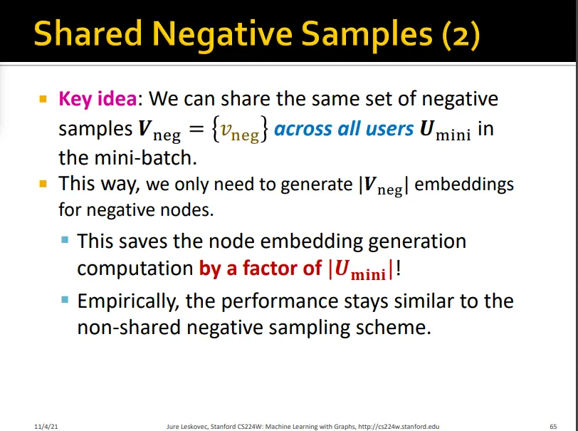
Shared Negative Samples
•
BPR loss의 경우 user마다 하나의 positive item과 negative item set을 샘플링해야 함
•
더 많은 negative를 샘플링할수록 성능은 좋아지나 expensive해짐
•
mini-batch 내에서 모두 같은 negative sample을 share하도록 함
•
성능은 비슷하게 유지됨
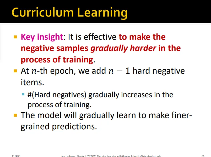
Curriculum Learning
•
학습이 진행될수록 더 어려운 학습셋을 제공
•
학습이 진행될수록 # hard negative sample을 더 추가함
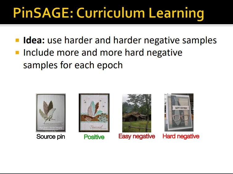
•
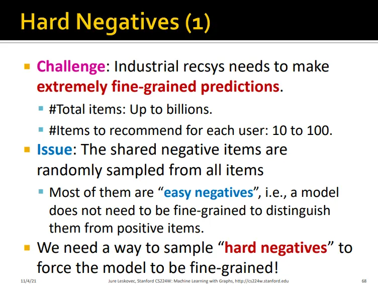
보통 item의 개수가 추천하는 item 개수에 비해 많기 때문에 negative를 샘플링해도 easy negative가 대부분임
•
모델이 fine-grained 되기 위해서는 hard negative가 필요함
•
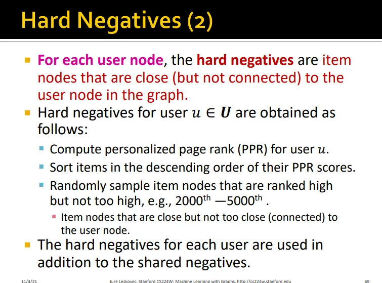
user에게 hard negative란 user와 그래프 상에서 가까우면서도 연결되어 있지는 않은 노드임
•
user의 hard negative를 구할 때는
1.
Personalized page rank를 계산함
2.
PPR score가 높은 샘플 중에서 랜덤으로 고름
•
PinSAGE는 rich node attribute과 graph structure를 활용해 high-quality embedding을 생성했을 뿐 아니라 negative sampling strategies를 통해 학습을 효율적으로 함