Recap: Deep Graph Encoders, GNNs

•
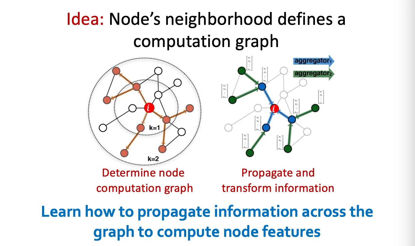
Aggregate Neighbors
Network에서 이웃과 일종의 computation graph가 형성되어 이웃의 정보를 aggregation 한다.
•
Why GNNs generalize other NNs?
GNN은 permutation invariance, equivariance의 개념이 적용된 형태로, CNN과 Transformer의 일반화된 형태로 볼 수 있다.
◦
CNN

Neighbor size가 고정되고 order가 정해진 GNN 형태이다.
◦
Transformer
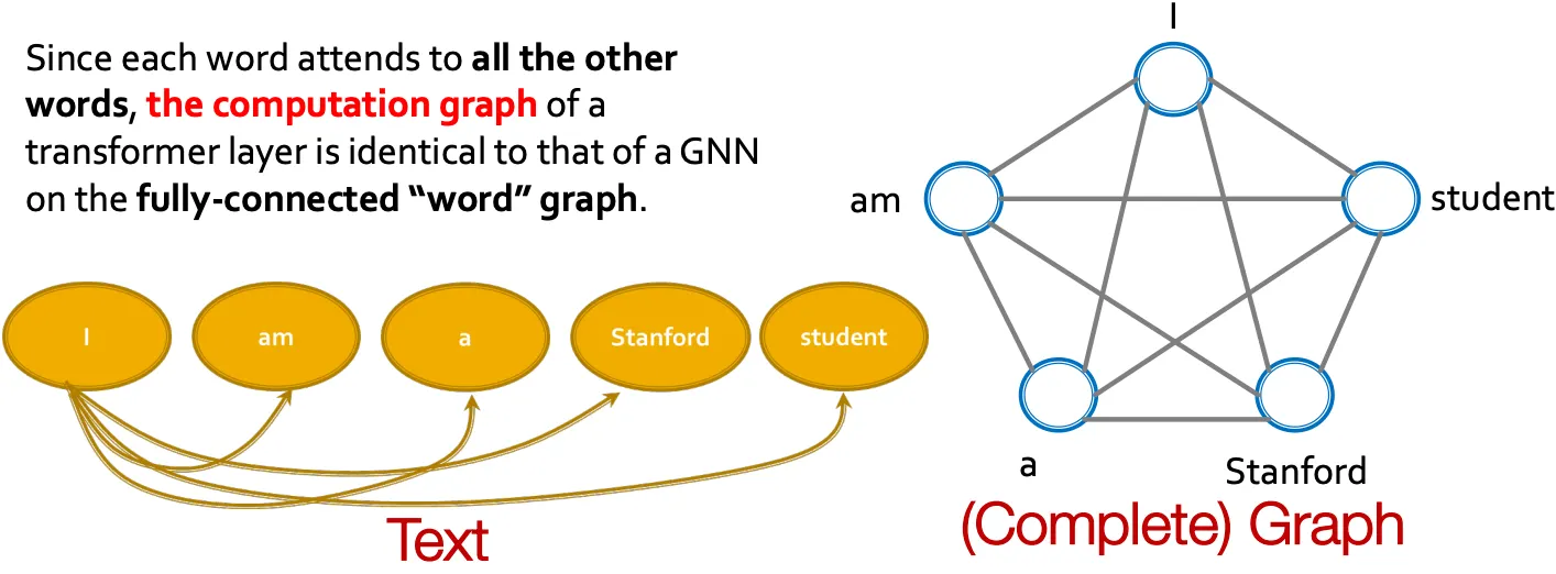
Fully-connected word graph라고 생각하면 transformer도 GNN의 일종이다.
A General Perspective on GNNs
•
GNN Framework

1.
GNN layer: Message
2.
GNN layer: Aggregation
e.g.) GCN, GraphSAGE, GAT, …
3.
Stacking layers
여러 layer를 이어 쌓고, skip connection을 넣는 방법
4.
Graph augmentation
•
Graph feature augmentation
•
Graph structure augmentation
5.
Learning objective
•
Supervised/Unsupervised
•
Node/Edge/Graph
A Single Layer of a GNN
•
GNN layer
Idea: Vector의 집합을 하나의 vector로 압축하는 것!
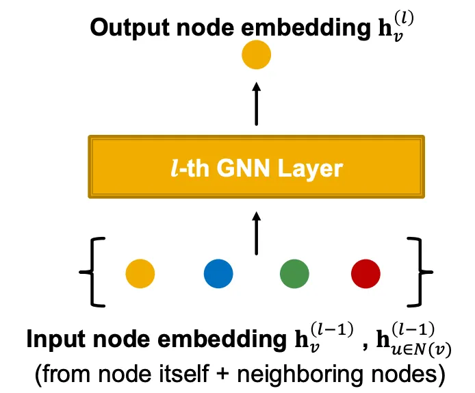
Two-step process:
1.
Message
각 node가 message를 만들고, 그 message가 나중에 다른 node 들로 전파된다.
Message functions
•
Linear layer 통과
2.
Aggregation
각 node가 주변 이웃 node들의 message를 aggregate 한다.
Aggregation은 order invariant 해야한다.
Aggregation functions
•
Sum/Mean/Max
•
Message Aggregation: Issue & Solution
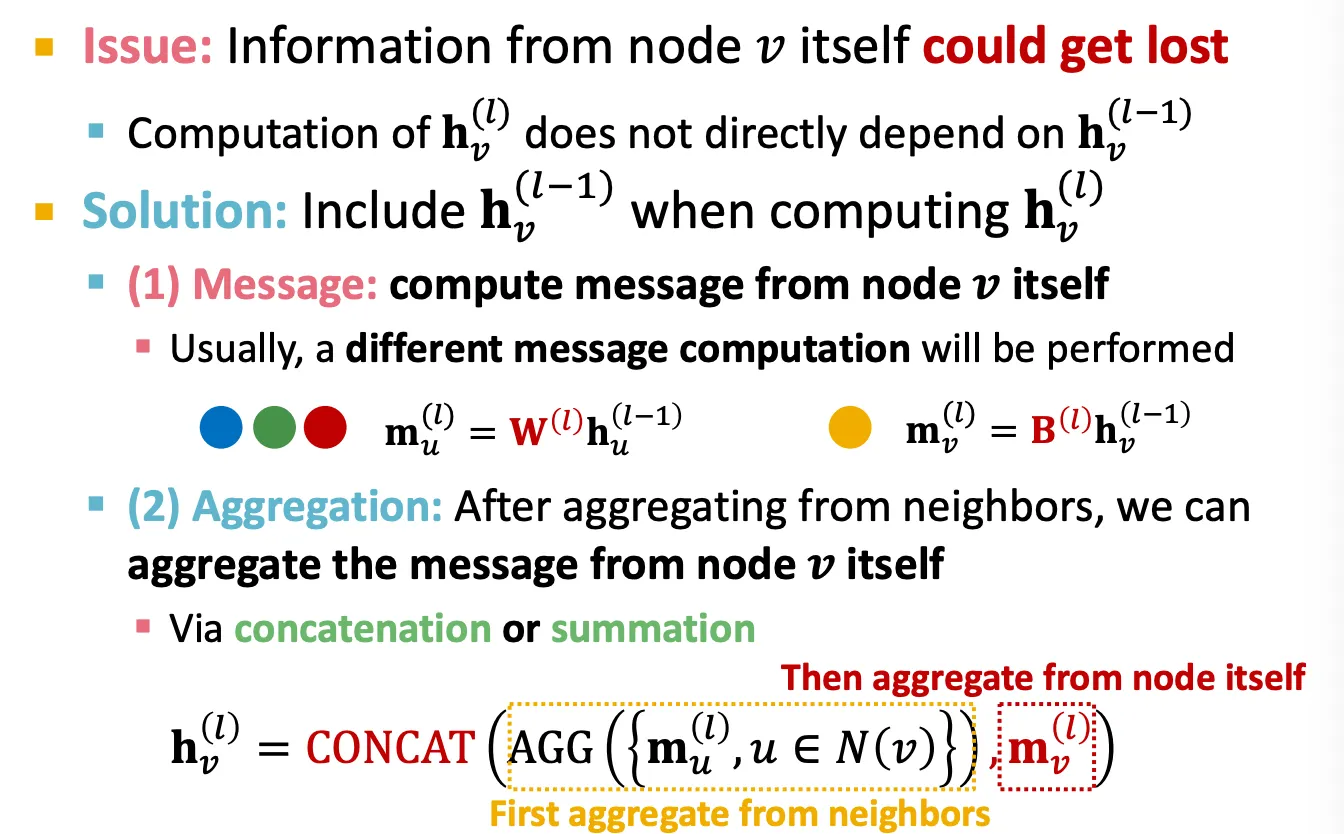
Issue: 이웃 node 들의 정보만 aggregate 하면 node 자신의 정보가 없어질 수 있다.
Solution: 를 계산할 때 도 사용한다.
1.
Message
,
보통 message computation은 neighbor와 self가 다른 weight parameter를 사용해 계산된다.
2.
Aggregation
Neighbor로부터 aggregate할 때 자신의 정보를 사용해서 concat 또는 sum 한다.
•
Putting this together
1.
Message
2.
Aggregation
3.
Non-linearity
Expressiveness를 위해 ReLU, Sigmoid 등을 사용한다.
Message 또는 aggregation에 사용할 수 있다.
•
Classical GNN Layers
◦
Graph Convolutional Networks (GCN)
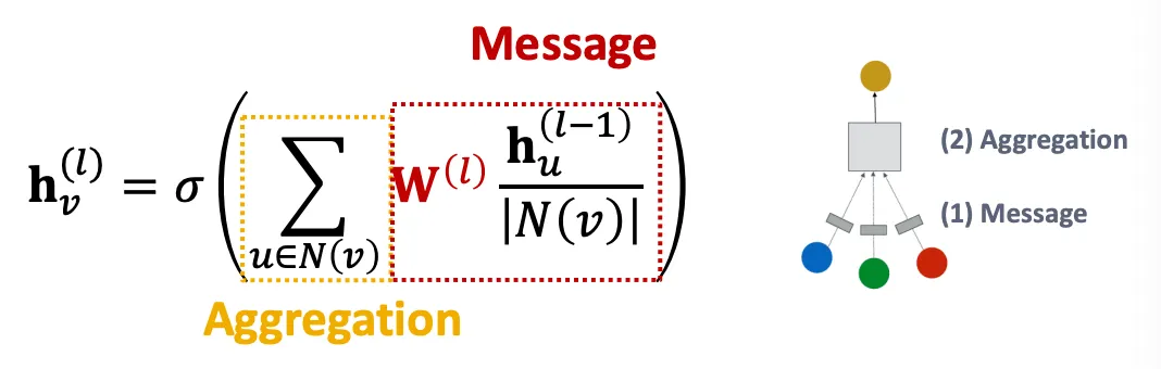
1.
Message
Weight matrix를 곱한 뒤 node degree로 normalize를 하여 각 node의 embedding을 만든다.
2.
Aggregation
이웃 노드로부터 sum을 하고, activation을 적용한다.
표현은 Sum 이지만, node degree로 normalize 하므로 결국 average 이다.
참고) GCN에서는 graph에 self-edge가 추가되어 있어, summation에 기본으로 포함된다.
◦
GraphSAGE
Two-stage aggregation
▪
Stage 1: Node neighbor로부터 aggregation
▪
Stage 2: 이후 자기 자신으로부터도 aggregation
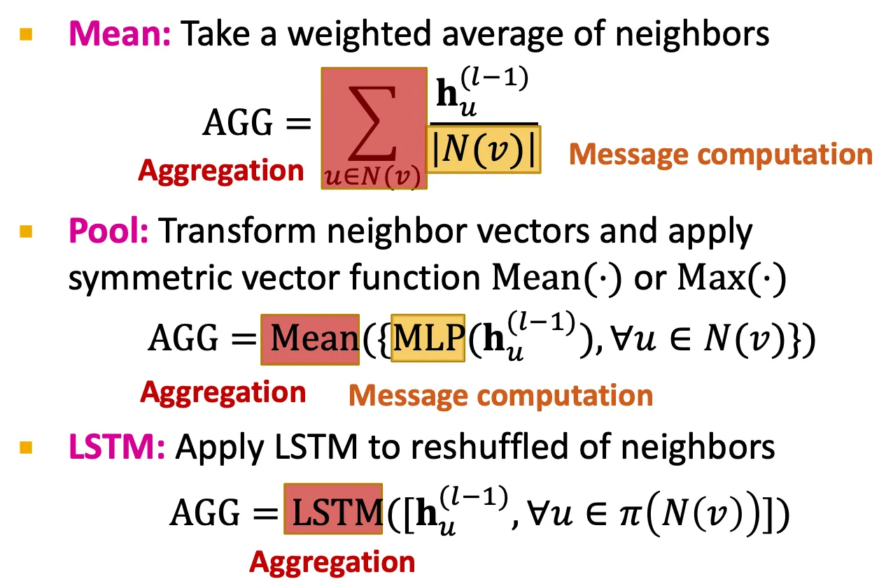
Aggregation 하는 방법은 Mean, Pool, LSTM 등을 사용할 수 있다.
참고) LSTM은 order가 있는 language model이기 때문에 order를 계속 shuffle해서 사용한다.
L2 normalization
모든 layer에서
Embedding vector를 L2 normalization으로 scaling 해준다.
◦
Graph Attention Networks (GAT)
▪
GCN, GraphSAGE에서는 aggregation 시에 모든 neighbor가 동일한 weight를 가져간다.
▪
하지만 GAT에서는 모든 node가 동일하게 중요하지는 않을 것이라는 intuition에 기반하여 attention을 적용한다.
▪
Attention mechanism
1.
Attention coefficient 가 아래와 같이 계산된다.
는 node 의 입장에서, node 의 중요도를 의미한다.
e.g.) attention의 형태 예시
•
..?
2.
Normalize →
3.
Weighted sum based on
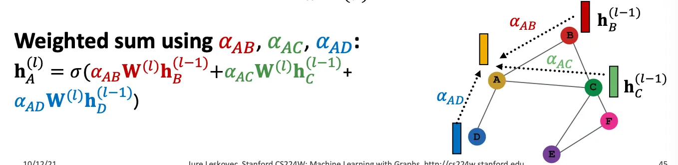
▪
Form of attention mechanism
다양한 attention mechanism을 사용할 수 있다.
e.g.) Simple single-layer neural network

Attention mechanism의 parameter는 함께(jointly) 학습된다.
▪
Multi-head attention
일종의 ensemble 개념으로 attention process를 안정화해준다.

GNN Layers in Practice
•
Classic GNN layer를 먼저 사용해보는 것이 좋은 시작 지점이다.
•
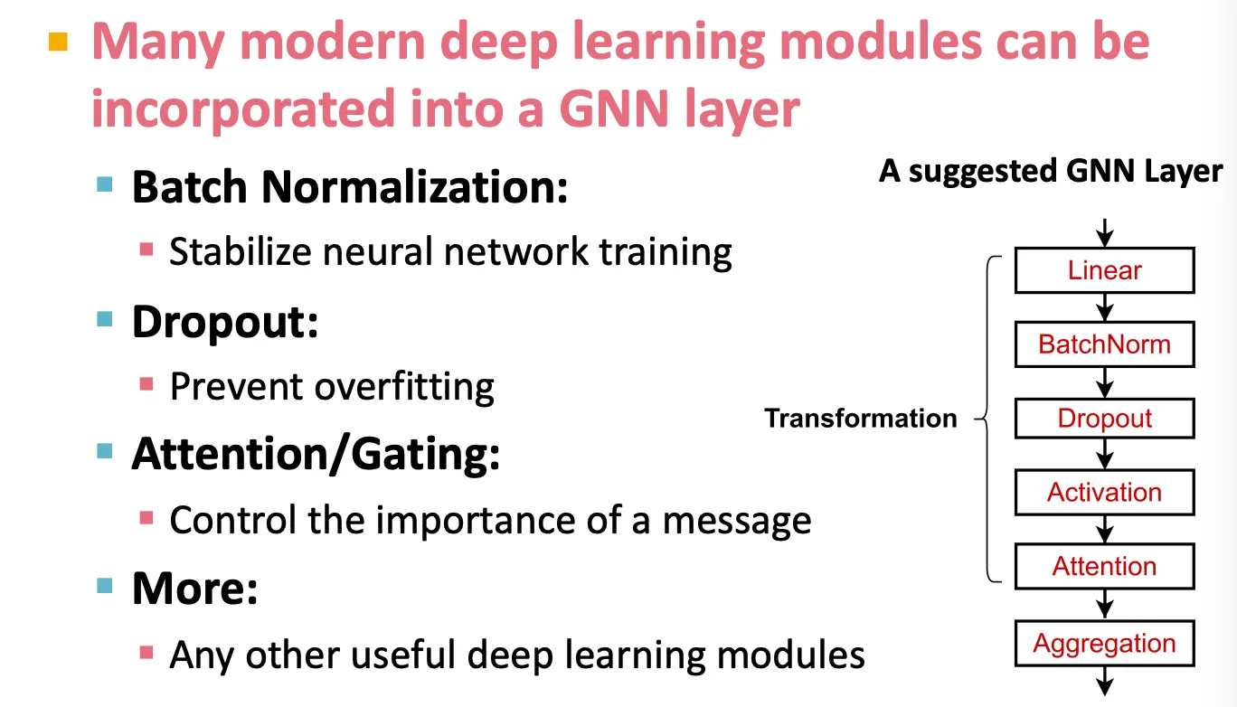
다양한 현재 deep learning technique을 GNN layer에 도입할 수 있다.
◦
Batch normalization

한 batch에 해당하는 input들에 대해 mean 과 variance를 계산하여, zero mean, unit variance의 분포를 띄도록 scaling을 해주는 방법으로, 학습을 안정화시켜준다.
◦
Dropout

Overfitting을 방지하는 방법으로, training 시에는 일정 비율만큼의 node를 turn-off 하고, test 시에는 모두 사용하는 방법이다.
GNN에 적용할 때는 주로 message function의 linear layer에 적용한다.
◦
Activation
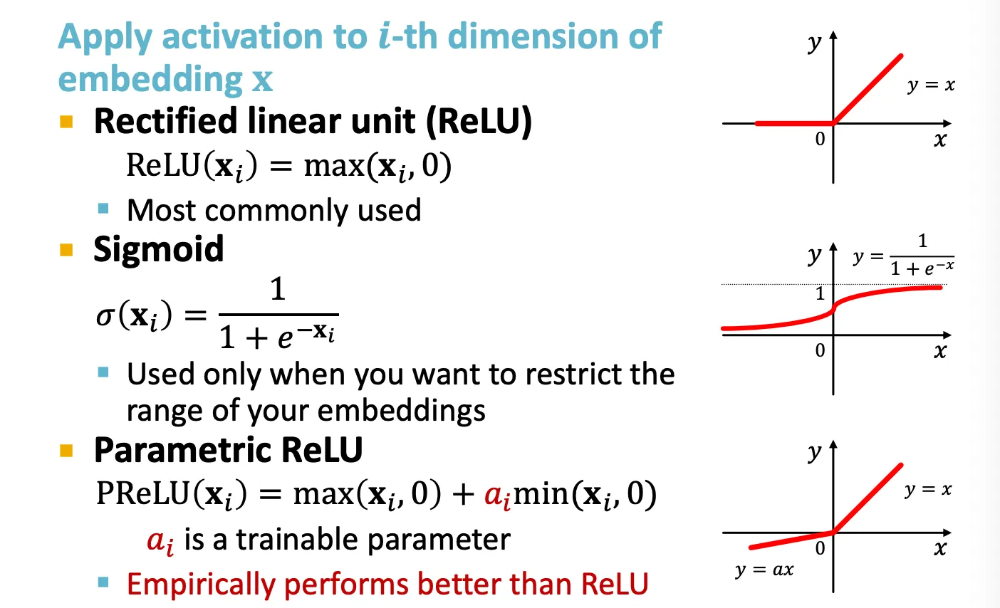
ReLU, Sigmoid, Parametric ReLU 등을 사용한다.
Stacking Layers of a GNN
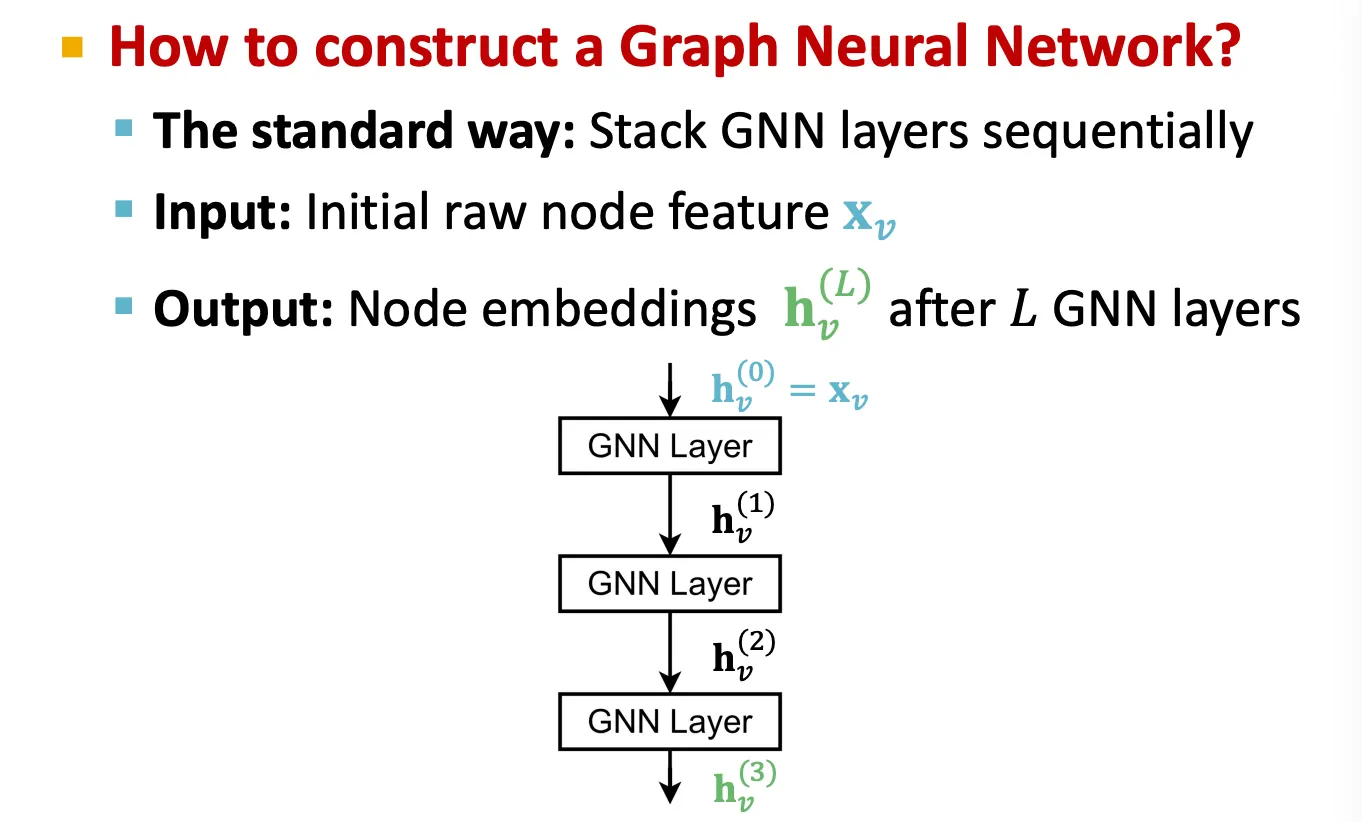
일반적으로, GNN layer를 쌓을 때는 순차적으로 여러 층을 쌓는다.
•
Oversmoothing
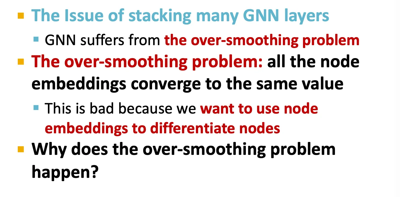
하지만 naïve한 방법으로 여러 층을 쌓으면 over-smoothing problem이 발생하는데, 이는 모든 node의 embedding이 비슷한 값으로 수렴하여 node 들을 구분할 수 없는 수준에 도달하는 현상이다.
•
Receptive field of a GNN
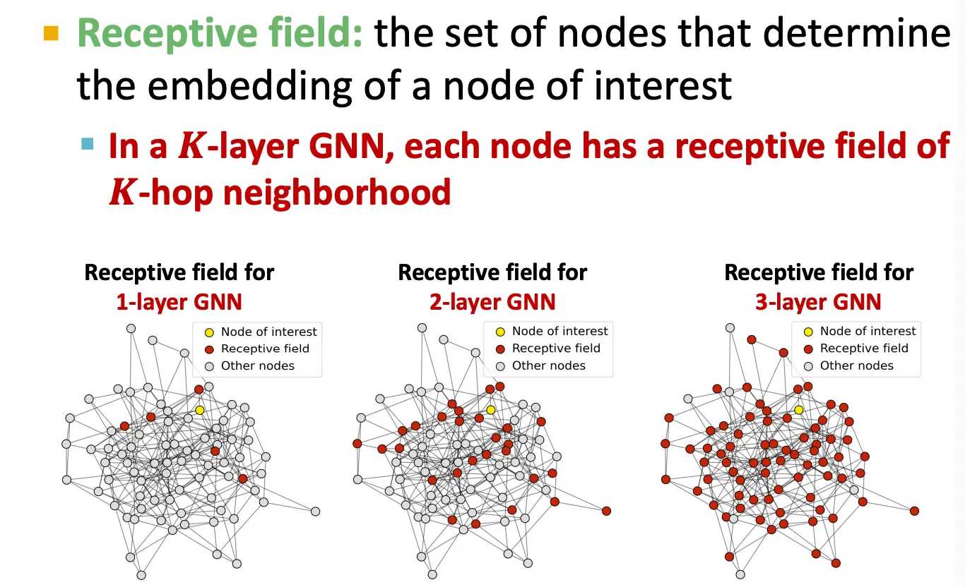
CNN에서와 비슷하게, GNN도 receptive field 를 정의할 수 있는데, 어떤 node에 대해 얼마나 주변 node를 볼 것인지를 의미한다.
-layer GNN에서는 receptive field 가 -hop 만큼의 이웃들이다.
따라서 깊게 쌓을 수록 거의 대부분의 node들의 정보를 aggregate 하게 된다.
•
Oversmoothing 문제를 극복하는 방법
◦
Receptive field
GNN layer를 쌓을 때는 일반적인 neural network (MLP, CNN 등)를 쌓을 때처럼 층을 단순히 쌓으면 안 된다.
Domain에 맞게, receptive field가 얼마나 필요할지 분석해서 사용한다.
◦
Expressive power
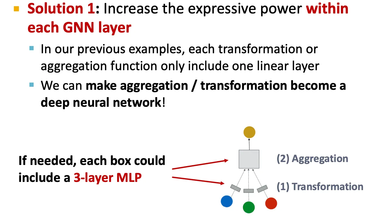
▪
GNN layer를 깊게 쌓지 말고, message function, aggregation function을 deep neural net으로 쌓아 expressivity를 높인다.
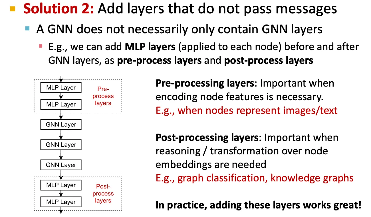
▪
GNN layer 사이에 pre-process, post-process layer를 쌓는다.
◦
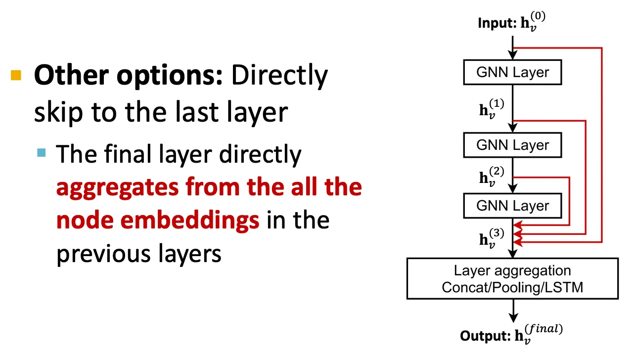
Skip-connection
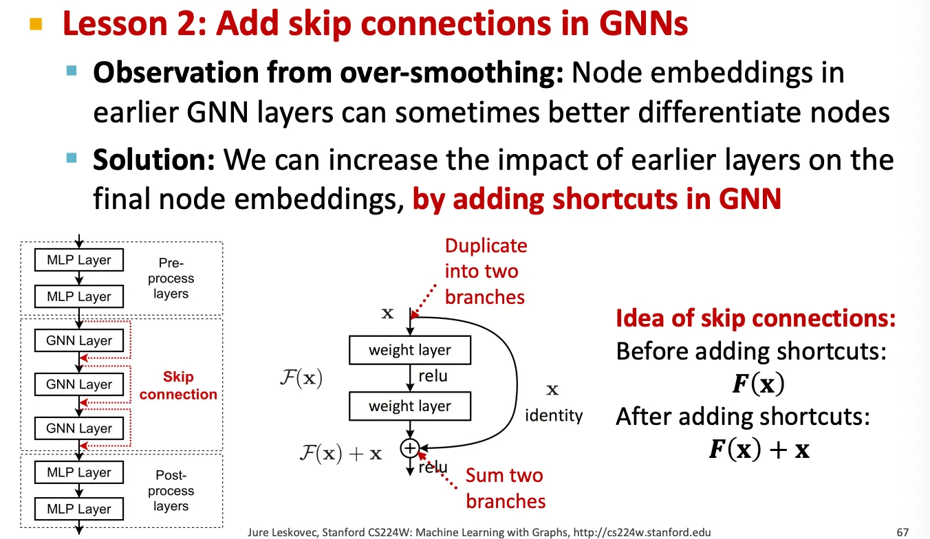
만약 GNN layer를 어쩔 수 없이 깊게 쌓아야 할 경우에는 skip connection을 이용해 앞 layer에서 얻은 embedding을 직접 더해서 사용해준다.
이 방법은 model을 mixture 형태로 사용하는 효과가 있다.
▪
Skip connection을 수행하는 방법은 크게 2가지가 있다.
1.
Vanilla skip connection

h 가 밖에 있으면 안 되나..?
2.
Jumping knowledge (맞는지 확인 필요)