

index

Abstract
With the recent success of graph convolutional networks (GCNs), they have been widely applied for recommendation, and achieved impressive performance gains.
The core of GCNs lies in its message passing mechanism to aggregate neighborhood information.
However, we observed that message passing largely slows down the convergence of GCNs during training, especially for large-scale recommender systems, which hinders their wide adoption.
LightGCN makes an early attempt to simplify GCNs for collaborative filtering by omitting feature transformations and nonlinear activations.
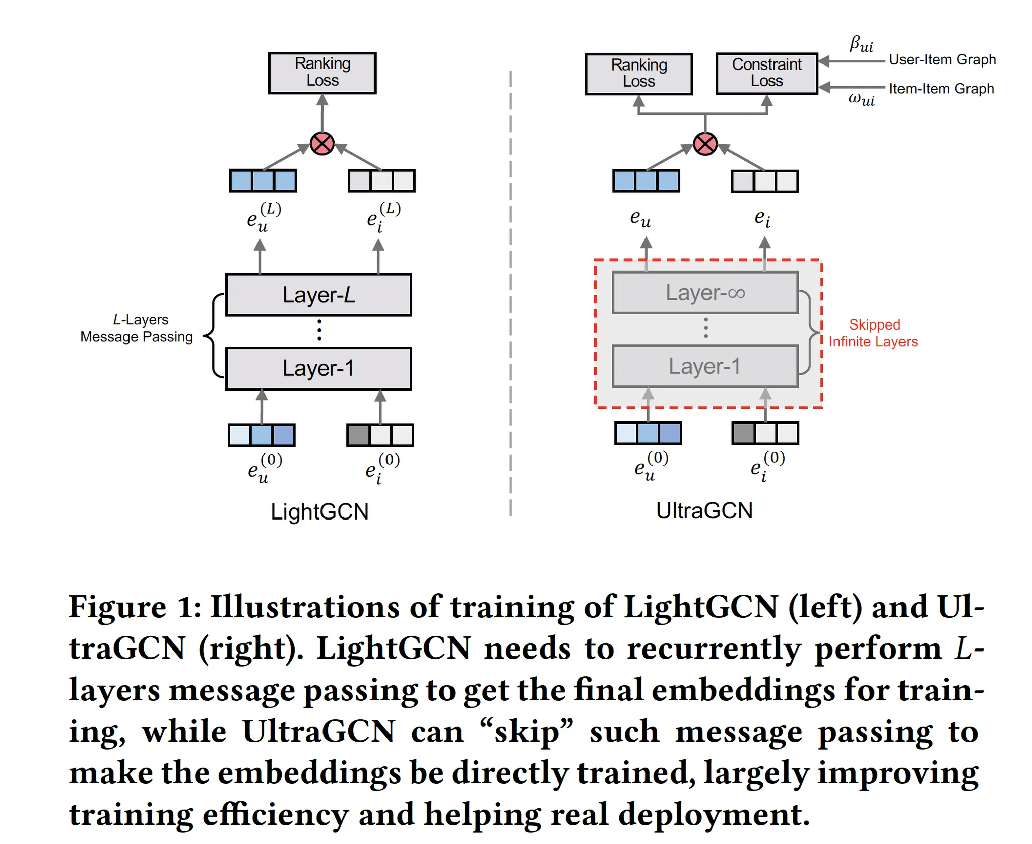
In this paper, we take one step further to propose an ultra-simplified formulation of GCNs (dubbed UltraGCN), which skips infinite layers of message passing for efficient recommendation.
Instead of explicit message passing, UltraGCN resorts to directly approximate the limit of infinite-layer graph convolutions via a constraint loss.
Meanwhile, UltraGCN allows for more appropriate edge weight assignments and flexible adjustment of the relative importances among different types of relationships.
This finally yields a simple yet effective UltraGCN model, which is easy to implement and efficient to train.
Experimental results on four benchmark datasets show that UltraGCN not only outperforms the state-of-the-art GCN models but also achieves more than 10x speedup over LightGCN.
GCN, LightGCN
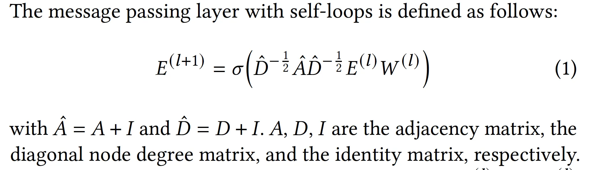
1. Message Passing in GCN[1]
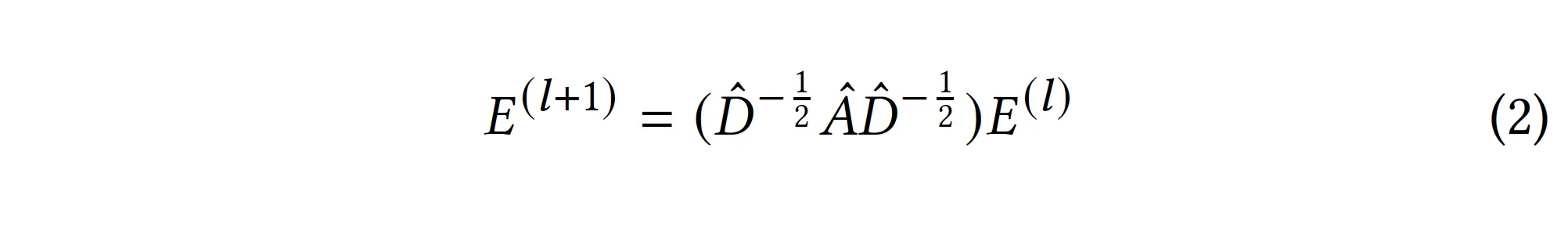
2. Message Passing in LightGCN[2]
•
GCN에서 아래의 항목들을 제거함
◦
feature transformation(W)
◦
nonlinear activation()
◦
self-loop connections(I) - 하지만 각 layer의 출력을 모두 사용해 final output을 만듦으로써 self-loop이 있는 것과 동일한 효과를 가짐
3. 2를 풀어서 쓰면…
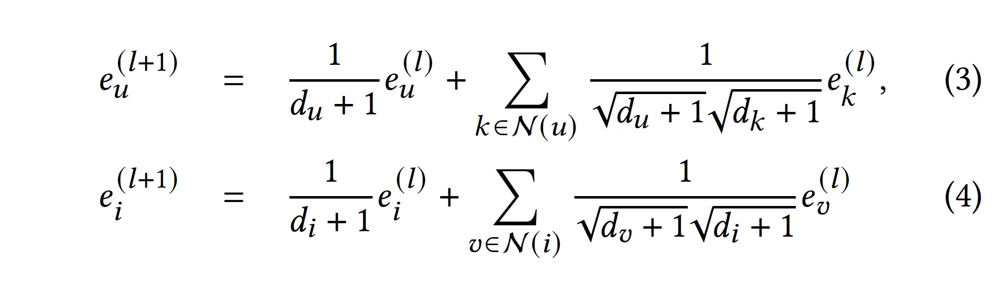
•
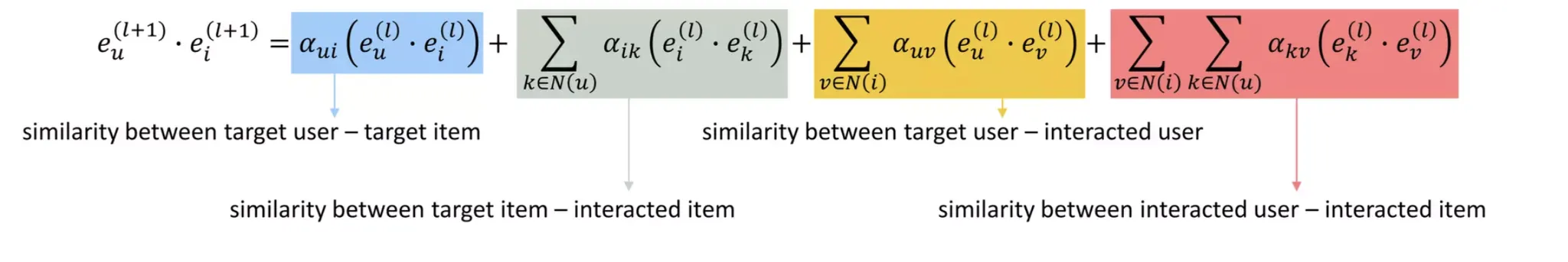
최종적으로는 와 의 dot product로 user-item edge를 예측하게 될 것이므로, 를 전개해 보면
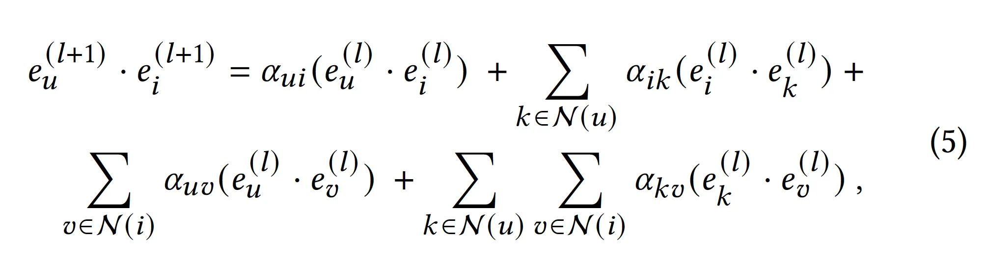

4. 3을 뜯어서 보면…[3]
•
네 가지 component로 분리됨
◦
target user - target item interaction
◦
target item - interacted item
◦
target user - interacted user
◦
interacted user - interacted item
위 GCN-based model의 세 가지 Limitations
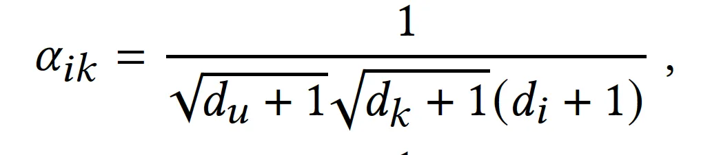
1. Item-item, User-user interaction factor의 비대칭성
•
item-item interaction factor
◦
interacted item k와 target item i 간의 가중치가 다름.
◦
i: (di + 1)
◦
k: sqrt(dk + 1)
•
user-user interaction factor에서도 동일
2. 서로 다른 interaction component의 가중치를 다르게 줄 수 없음
•
위의 네 가지 interaction component들이 최종 output에 주는 가중치를 바꿀 수 없음
•
레이어들을 쌓다 보면 별로 중요하지 않은 interaction component들이 포함될 수 있는데, 이는 학습의 효율성을 크게 저하함
•
It is desirable to flexibly adjust relative importances of various relationships.
3. Over-smoothing problem
•
이상적으로는 레이어를 더 많이 쌓을수록 high-order collaborative signal들이 반영되어 성능이 올라야 하나, 실제 LightGCN 등에서 레이어 2~3개만 쌓아도 성능이 떨어지기 시작함.
•
이건 over-smoothing 문제에 기인하는 부분도 있는데, layer을 많이 쌓을 수록 same-degree를 갖는 노드들이 점점 동일하게 임베딩됨
UltraGCN
•
기존 GCN들은 user, item 임베딩들을 l개의 message-passing layer을 통과시켜 embedding refine한 후 이들을 dotprod한다
•
UltraGCN은 message-passing layer를 없다(=모델 구조는 Matrix Factorization과 완전 동일!). 대신 그래프 구조를 반영한 constraint loss가 loss 항에 추가된다.
•
constraint loss는 어떻게 만들어지나? → message passing이 완전 잘 되었을 때 임베딩들 간에 가질 ideal한 관계들을 현재 임베딩들이 갖도록 한다.
1. User-Item graph의 반영
•
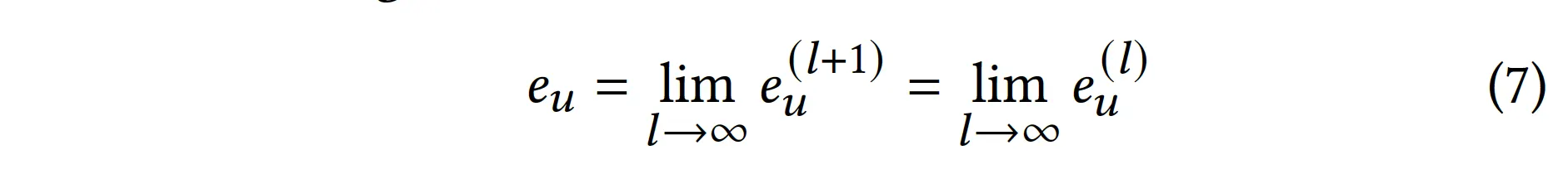
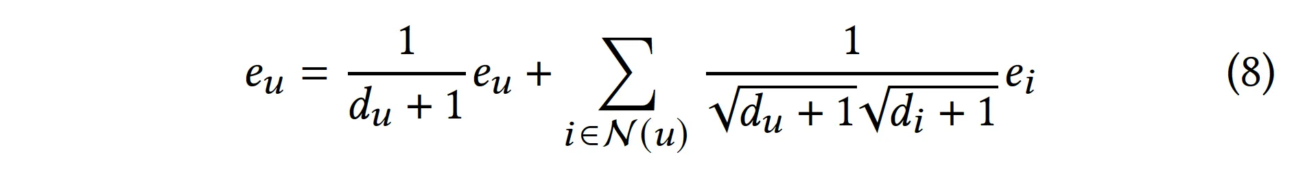
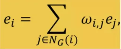
infinite layer을 통과하여 message passing이 완벽하게 이루어졌다면, 유저 임베딩의 최종 수렴 상태는 다음과 같다.
•
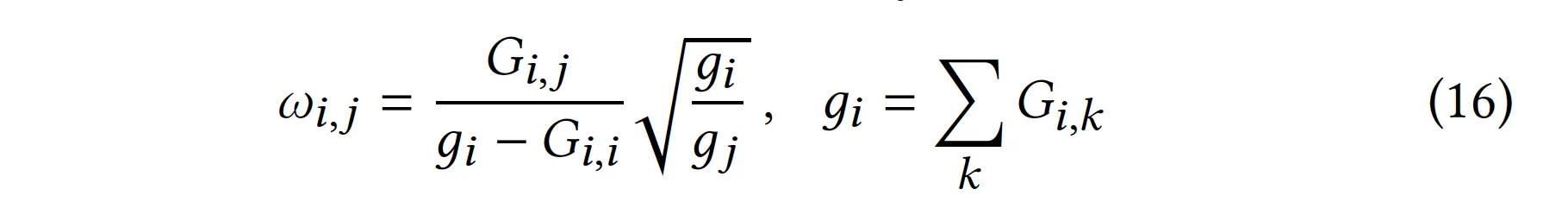
근데 message passing은 아래 관계를 갖는다.
•
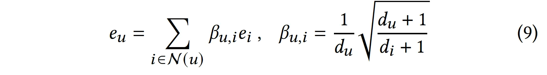
식 7, 8을 정리하면 아래와 같다.
•
즉 9번 식의 상태를 만족한다면 message passing이 완벽하게 이루어진 것.
•
9번 식의 상태가 되도록 loss를 구성하자. 즉, 9번 식의 좌우 항이 유사해지도록 loss를 구성하자.
◦
Trick: 각 임베딩들을 unit vector로 normalize한다.
◦
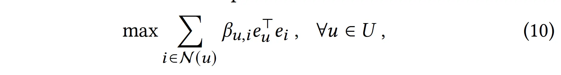
그러면 아래 식이 좌우 항의 유사도이다(cosine similarity between and )
•
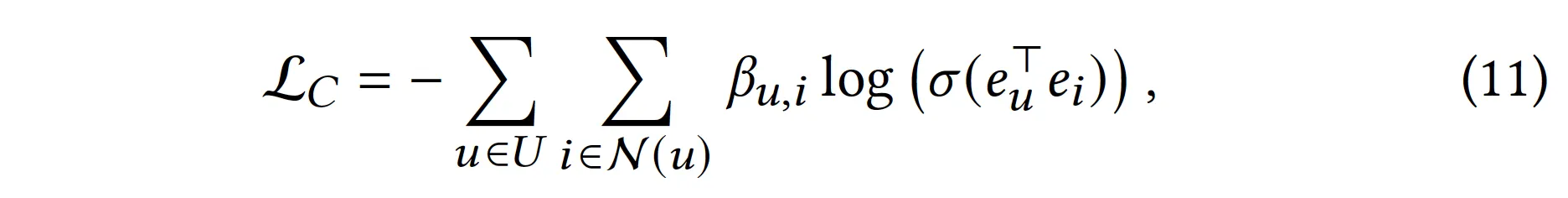
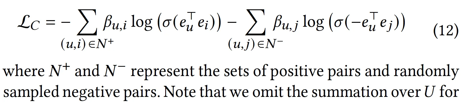
최적화에서의 편의성을 위해 sigmoid를 씌우고 nll-loss로 아래와 같이 구성하였다.
•
근데 11번 식은 over-smoothing 문제를 겪게 된다. 모든 인 , 쌍에 대해 임베딩이 동일해질 때 극소를 갖기 때문 → negative sampling을 통해 해결하자.
•
최종 Loss에는 어떻게 반영?
◦
Task loss는 pairwise BPR vs pointwise BCE로 설정됨
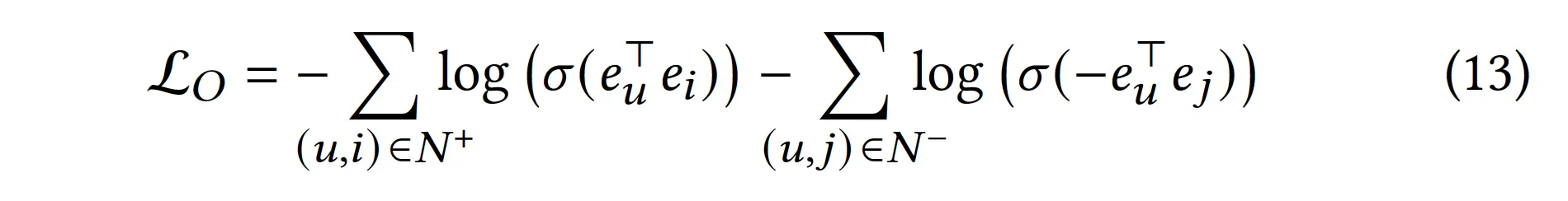
◦
최종 loss는 task loss + weighted constraint-loss
▪
Note: Lo와 Lc는 식의 구조가 동일하긴 하지만. Lo와 Lc에 사용되는 negative sample은 다를 수도 있음(nsrate=300)

2. Item-Item graph의 반영
1.
Item-Item Co-occurance graph 생성

2.
User-item graph에서와 똑같은 방법으로, 그래프 G에서 ideal state를 approximate할 수 있는 loss function을 생성
a.
user-item graph의 == item-item graph의
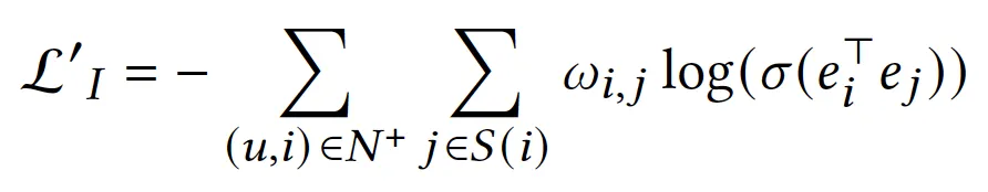
b.
item-item connection의 sparsity를 보장하고 학습 효율을 늘리기 위해, item-item graph에서는 각 아이템 i에 대해 기준 상위 K개의 유사 아이템만 선택하여 loss에 더함(N(i) → S(i), |S(i)|=K)(학습에서는 K=10)
c.
(Lo, Lc에서의 negative sampling이 이미 충분히 over-smoothing을 극복하게 도와주므로 여기서는 굳이 negative sampling 하지 않았다고 함)

3.
최종 Loss?

Note) Flexibility
•
LightGCN에서는 U-I, I-I interaction의 가중치를 따로 조절할 수 없었음
•
UltraGCN에서는 message passing이 없이 각 interaction을 loss function에 따로 반영하기 때문에, loss function에서의 가중치를 조절함으로써 해당 interaction의 임팩트를 유연하게 조정할 수 있음
•
또한 U-I, I-I가 아니더라도 여러 Interaction(ex: social graph에서의 u-u, knowledge graph 등~)을 loss에 반영함으로써 학습에 반영할 수 있음
성능
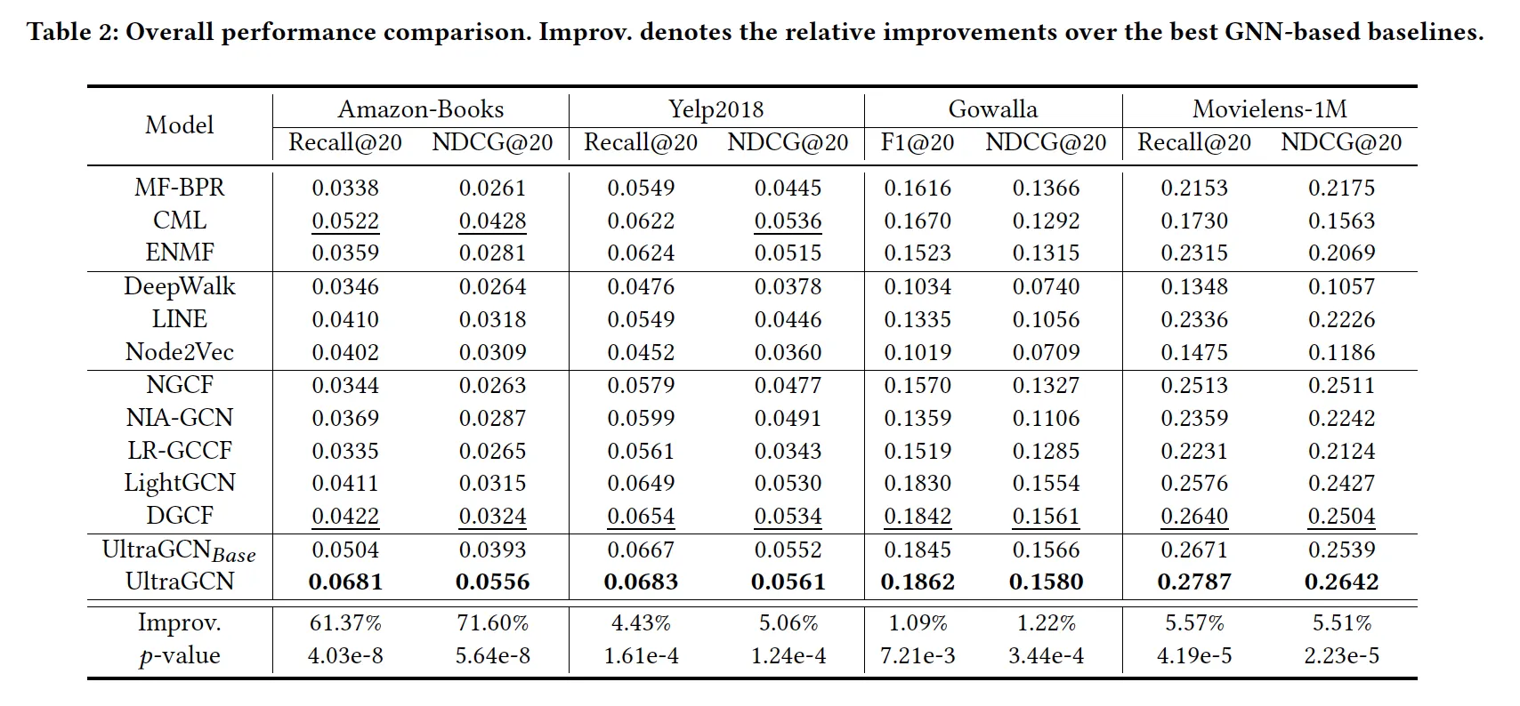
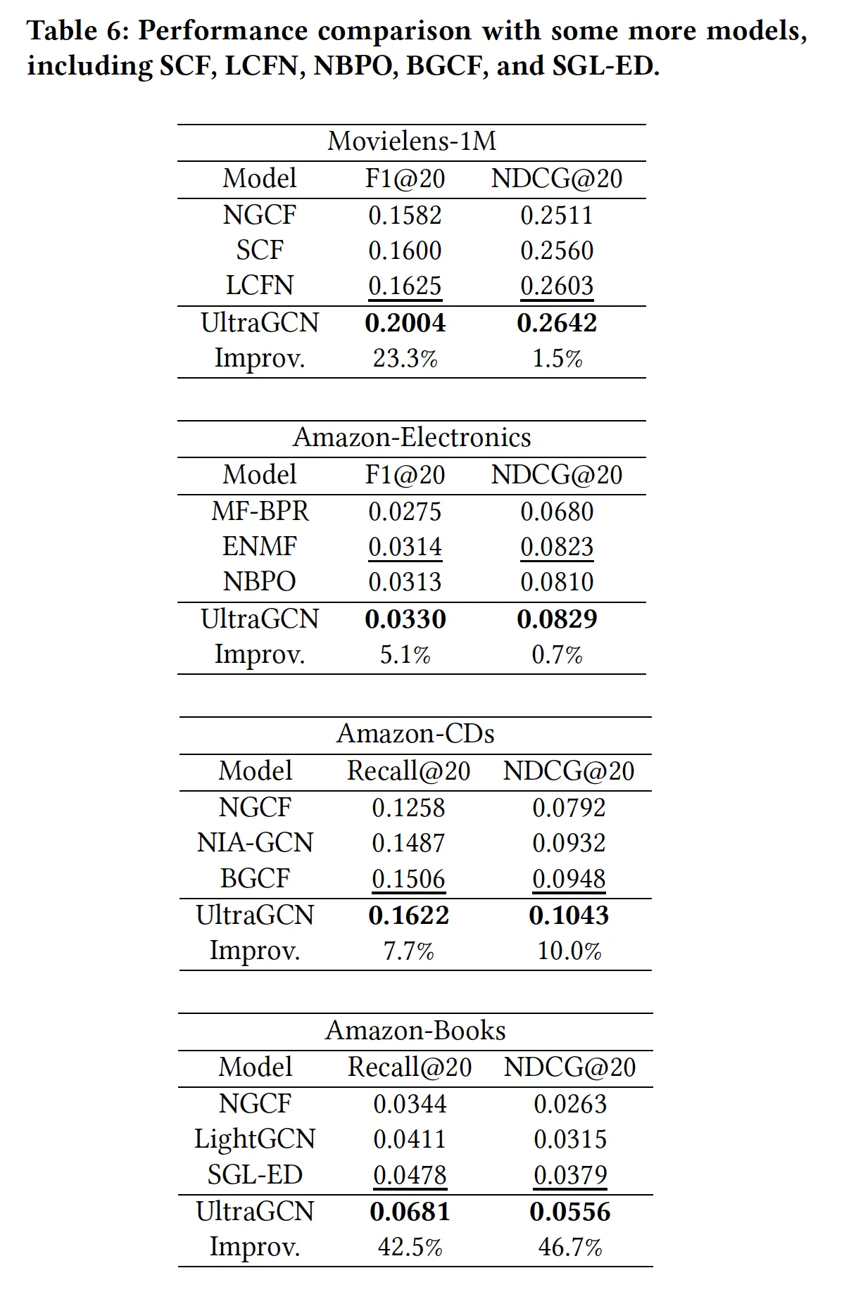
1. Performance
•
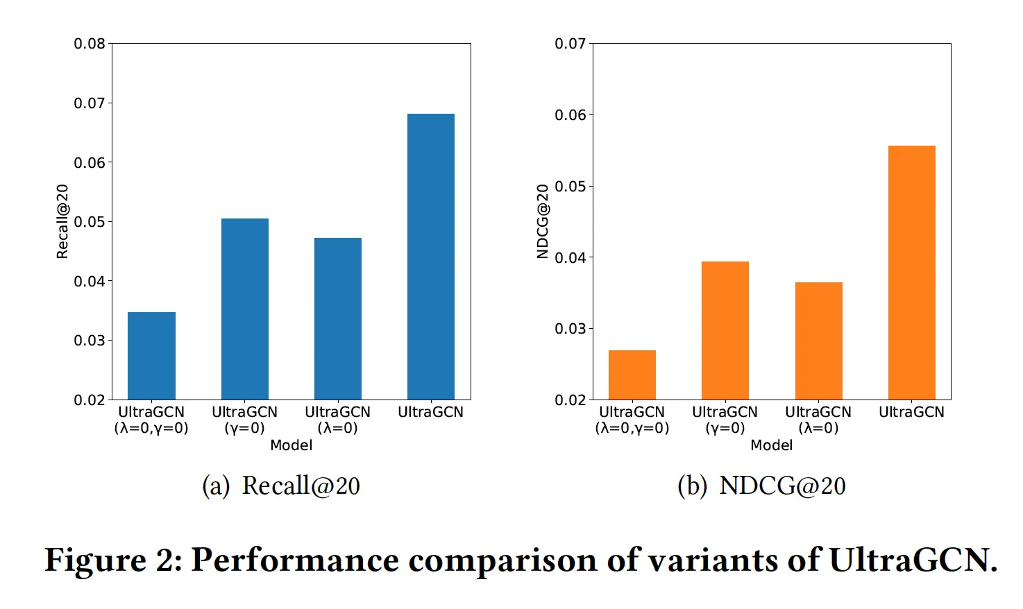
UltraGCN-base: item-item graph가 반영되지 않은 모델
•
네 개의 데이터셋에서 일관적으로 UltraGCN이 다른 모델보다 우수한 성능을 보임. 왜일까?
1.
U-I, I-I graph에 부여한 가중치들이 적절했고(thx to flexibility), 값에 따라 / top-K개 i-i graph neighbour을 선택하는 과정 덕에 불필요한 interaction이 잘 필터링되었다.
2.
UltraGCN이 graph convolution의 본질만 효율적으로 잘 사용하여, deep collaborative signal을 잘 반영했다.
•
또 다른 장점: UltraGCN은 모델 구조는 본질적으로 MF와 동일하고 loss만 바뀌는 것이므로, DGCF같은 sota MF 모델들에도 orthogonal하게 적용 가능하다. 갖다붙이면 성능 더 오를걸?
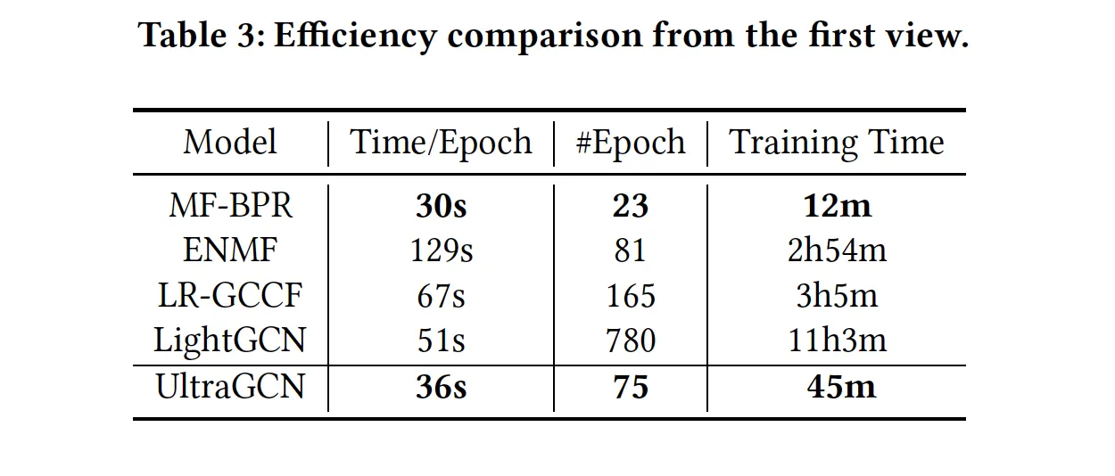
2. Efficiency
•
Table 3: 최고 성능을 달성하기까지 몇 epoch이 걸리나? epoch당 학습 시간은? 총 학습 시간은?
◦
MF-BPF이 가장 빠르고 그 다음이 UltraGCN(하지만 두 모델의 성능 차이는 매우 크다).
•
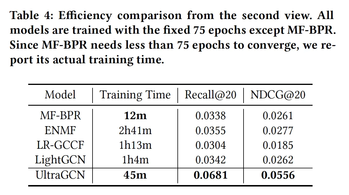
Table 4: 75 epoch 학습까지 얼마나 걸리고 성능은 어느 정도?
◦
UltraGCN이 best
3. Ablation study(Amazon-Book)
•
U-U 그래프는 왜 안 써? → 써봤는데 크게 성능 차이 없어서

•
U-I, I-I 둘다 성능에 중요한 것 맞아? → Yes. 근데 U-I가 I-I보다 더 중요한 듯
•
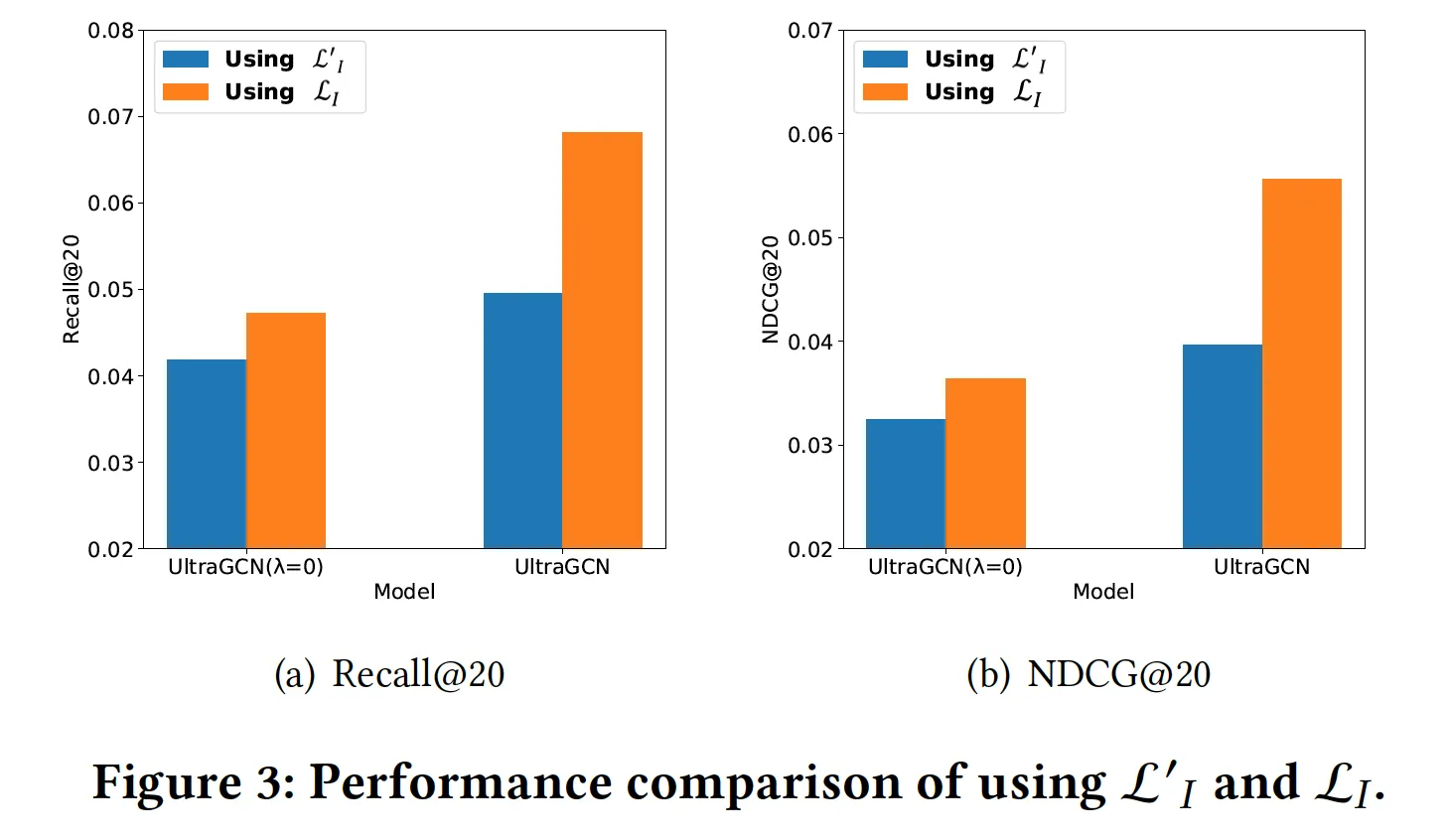
I-I graph 반영할 때, I-I graph에서의 U-I pair을 loss에 썼던데, I-I graph에서의 I-I pair을 반영하는 것보다 그게 낫나?
◦
L_I → L’_I로 바꿔서 실험해봤는데, 성능이 떨어짐

4. 파라미터 분석
•
K
◦
K가 너무 작으면 I-I graph를 충분히 활용하지 못하고, 너무 크면 noise가 많이 들어온다.

•
, (Amazon-Book)
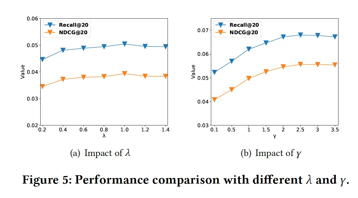
•
최적화 순서: 감마=0일 때 람다 최적화 → 람다 최적일 때 감마 최적화
•
둘다, 값들이 너무 작으면 그래프 요소를 학습에 충분히 반영하지 못해 성능이 떨어진다.
References
[1] Semi-Supervised Classification with Graph Convolution Networks(ICLR’17)
[2] LightGCN: Simplifying and Powering Graph Convolution network for Recommendation(SIGIR’20)
•
중요한 것은 본질. 그래프 구조를 사용하는 최종 목적은 연결된 노드 임베딩을 비슷하게 만드는 것 → 귀찮게 layer 통과시키지 말고, loss에서 직접 학습에 반영