

Deep Generative Models for Graphs
그 동안은 Graph에서 학습하는 문제에 대해 다뤘다.
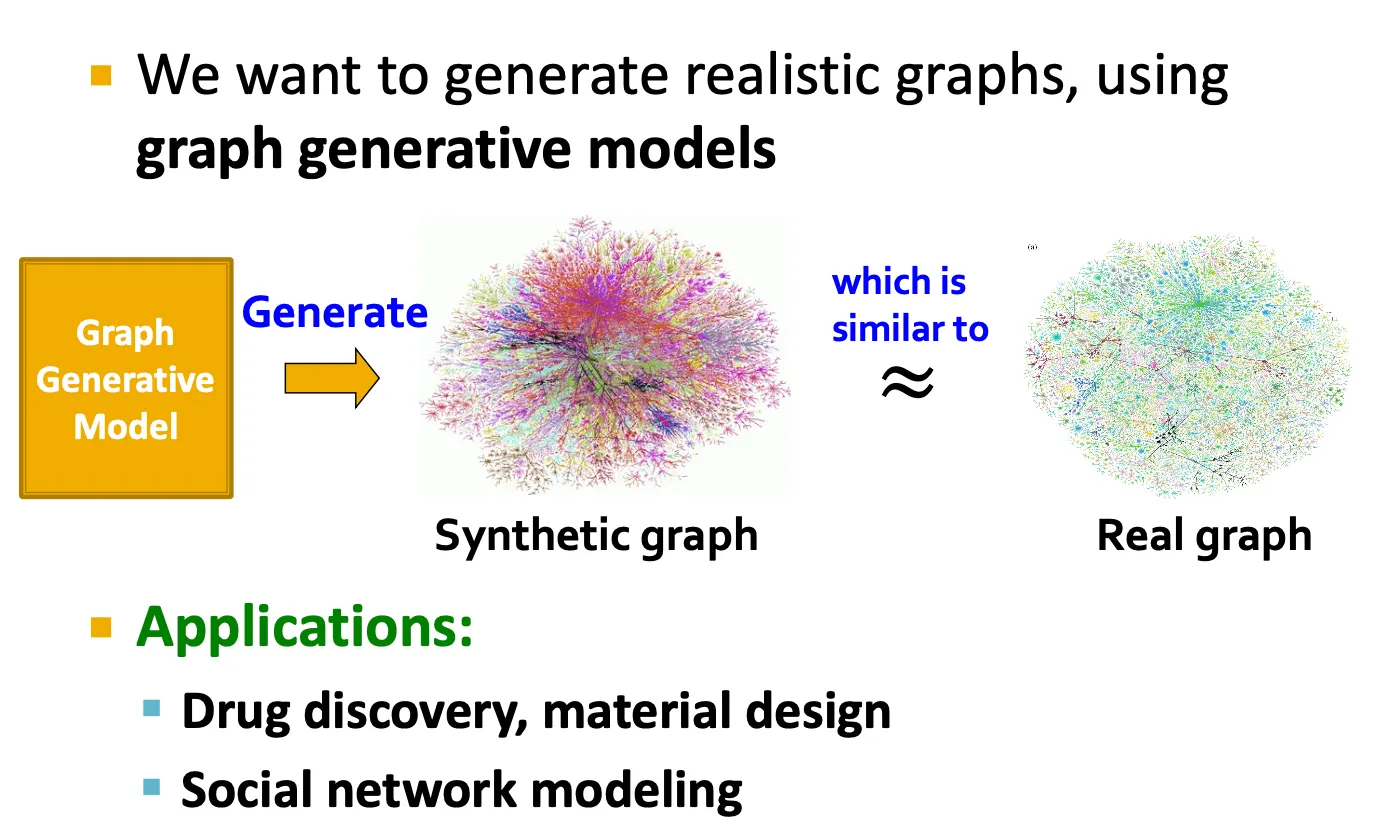
Graph generation
•
그런데 이런 graph들이 어떻게 만들어지는걸까?
•
Graph generation은 drug discovery, social network modeling 등에 적용할 수 있다.
Graph generation을 공부하는 이유
•
Insights: graph formulation에 대한 이해
•
Predictions: graph가 어떻게 바뀔지 예측.
•
Simulations: 일반적인 graph instance에 대해 simulation.
•
Anomaly detection: graph가 normal / abnormal 인지 결정.
Graph generation의 역사
1.
Real-world graph의 특성 이해
좋은 graph generative model은 real-world graph의 특성을 잘 반영해야 한다.
2.
전통적인 graph generative models
전통적인 model들은 어떤 assumption에 기반하여 생성한다.
3.
Deep graph generative models
Data로부터 graph formation process를 학습한다.
→ Lecture 15은 이 부분에 대해 다룬다.
Graph generation = Graph decoders!
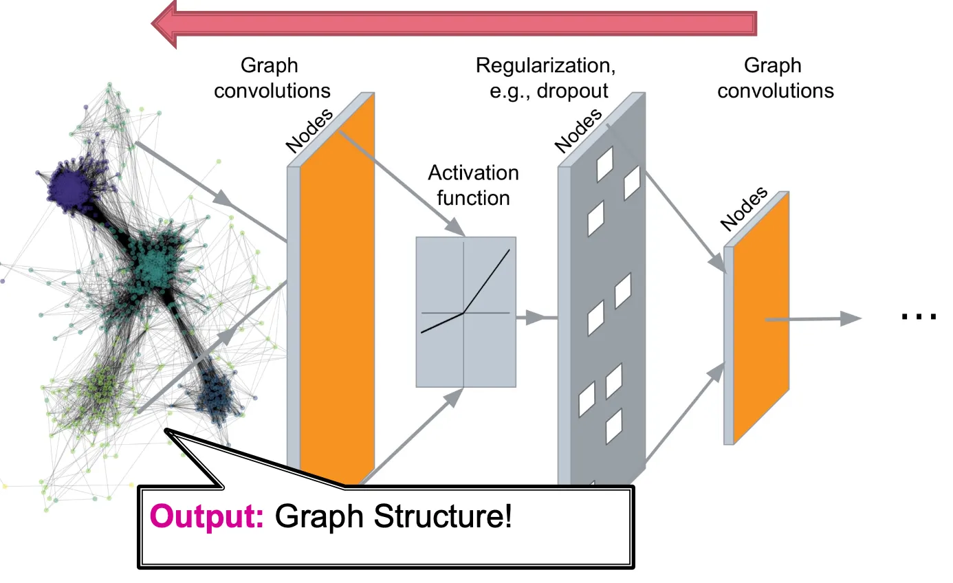
Machine Learning for Graph Generation
Graph generation tasks: 크게 두 가지로 나뉜다.
•
Task 1: Realistic graph generation
주어진 graph data와 유사한 형태의 graph를 생성하는 task. (Lecture 15에서 주로 다루는 내용)
•
Task 2: Goal-directed graph generation
어떤 objective나 constraint를 만족하는 graph를 생성하는 task.
e.g.) 어떤 물성을 가지도록 약물 generation
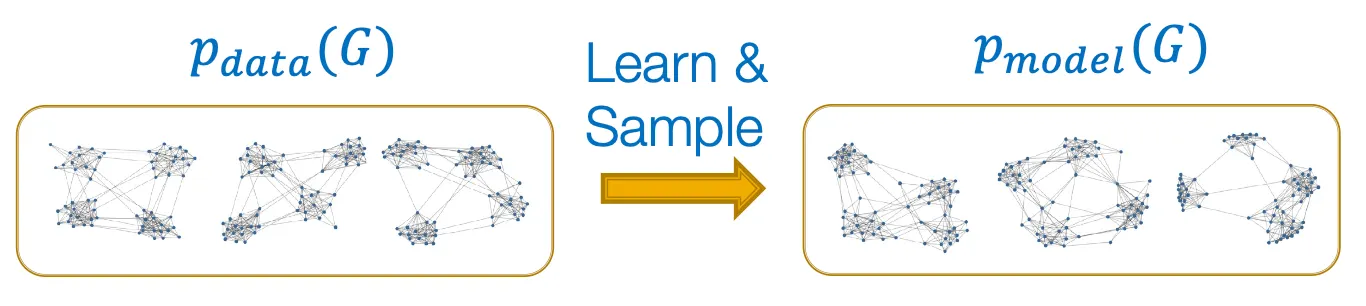
Graph generative models
•
기본적으로 MLE (maximum likelihood estimation) 이다.
•
Setup
◦
: data distribution (알려지지 않았고, 알 수도 없지만 에서 sampling 된)
◦
: model, parametrized by → approximation에 사용.
•
Goal
1.
Density estimation
를 에 비슷하도록!
2.
Sampling
에서 sampling하여 graph 생성!
Density estimation
•
Key principle: Maximum Likelihood
즉, data 를 만들어 냈을 것 같은 model을 찾는 것이 목적이다.
Sampling
•
어떤 complex distribution에서 graph sampling을 하는 단계.
1.
Simple noise distribution에서 sampling
2.
어떤 함수 에 의해 noise를 transform
이때 는 deep neural network를 사용해 학습한다.
Auto-regressive model
는 density estimation과 sampling 모두에 사용한다.
Chain rule에 의해, joint distribution은 conditional distribution의 product이다.
는 node를 추가하고, edge를 추가하는 번째 action 이다.
GraphRNN: Generating Realistic Graphs
Idea
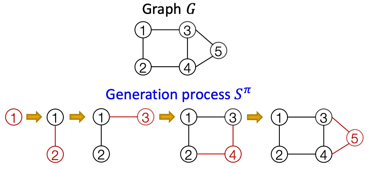

node와 edge를 순차적으로 추가하면서 graph를 generate.
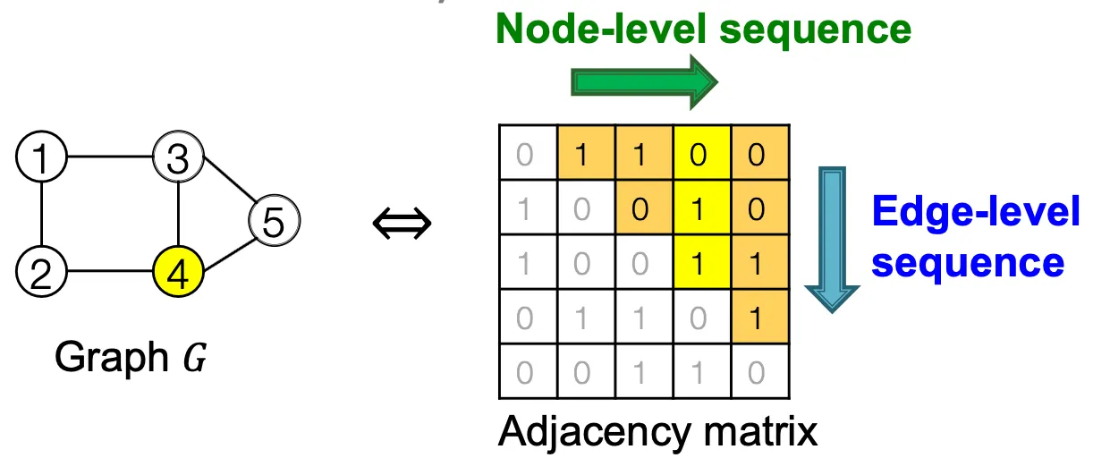
Graph를 sequence로 modeling - Two level approach
Node-level / Edge-level
Node-level RNN이 edge-level RNN을 위한 initial state를 만들어 준다.
Edge-level RNN은 순차적으로 새로운 node가 다른 이전의 node들과 연결될지 안 될지를 예측한다.
•
Node level
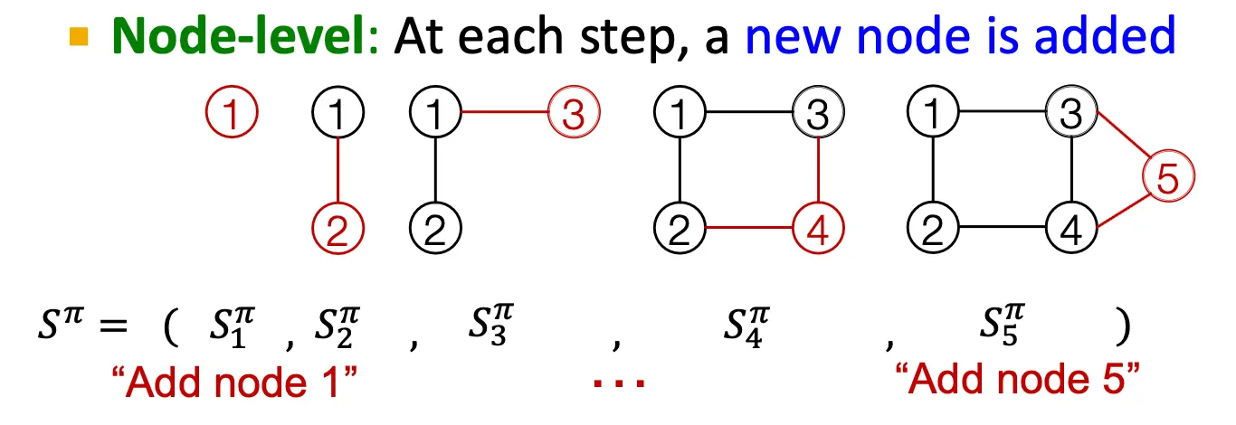
Node를 하나씩 추가한다.
•
Edge level

존재하는 node들 간에 edge를 추가한다.
Graph RNN Overview
•
즉, 어떤 graph에 node ordering을 부여하면, sequence의 sequence 형태로 생각할 수 있다.
•
GraphRNN에서는 node ordering이 random하게 부여된다.
•
Node level, edge level의 two step approach이다.
Background: RNNs
•
RNN은 sequential data를 위해 만들어진 모델이다.
•
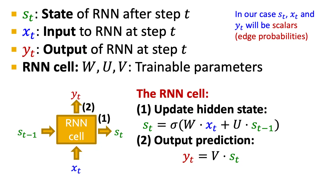
Input sequence를 순차적으로 받아서 hidden state를 update하고, 그 hidden state가 다음 cell로 전달된다.
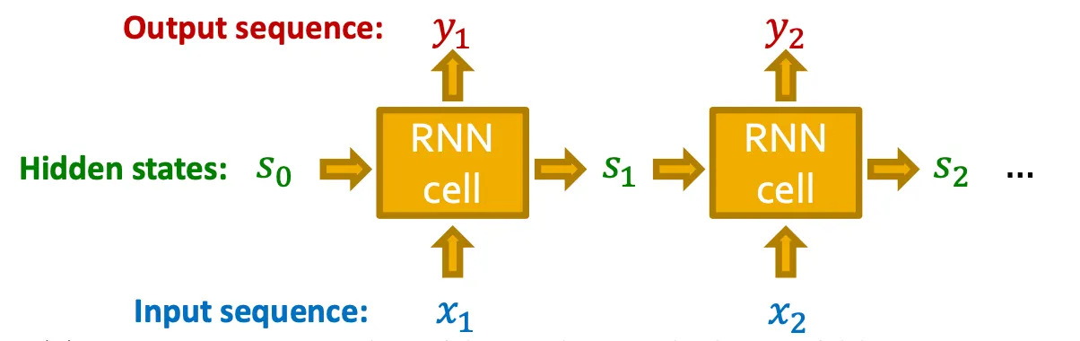
cf) Vanilla RNN보다 expressive한 cell은 GRU 또는 LSTM 등을 사용할 수 있다.
GraphRNN: Two levels of RNN

GraphRNN: Sequence Generation
•
Deterministic way
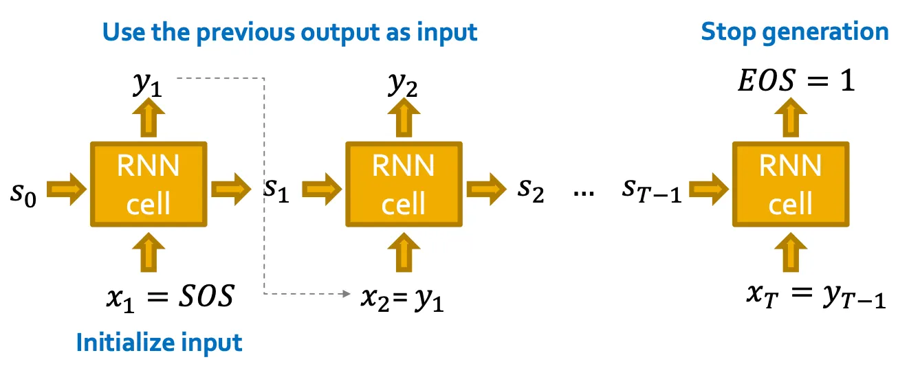
이전 cell의 output을 다음 cell의 input으로 사용하여 generation 할 수 있다.
하지만 이 방법은 deterministic 하다.
•
Stochastic way
우리의 목표는 를 modeling 하는 것이다.
따라서, 을 에서 sampling 해서 사용할 수 있다.

◦
Test time strategy
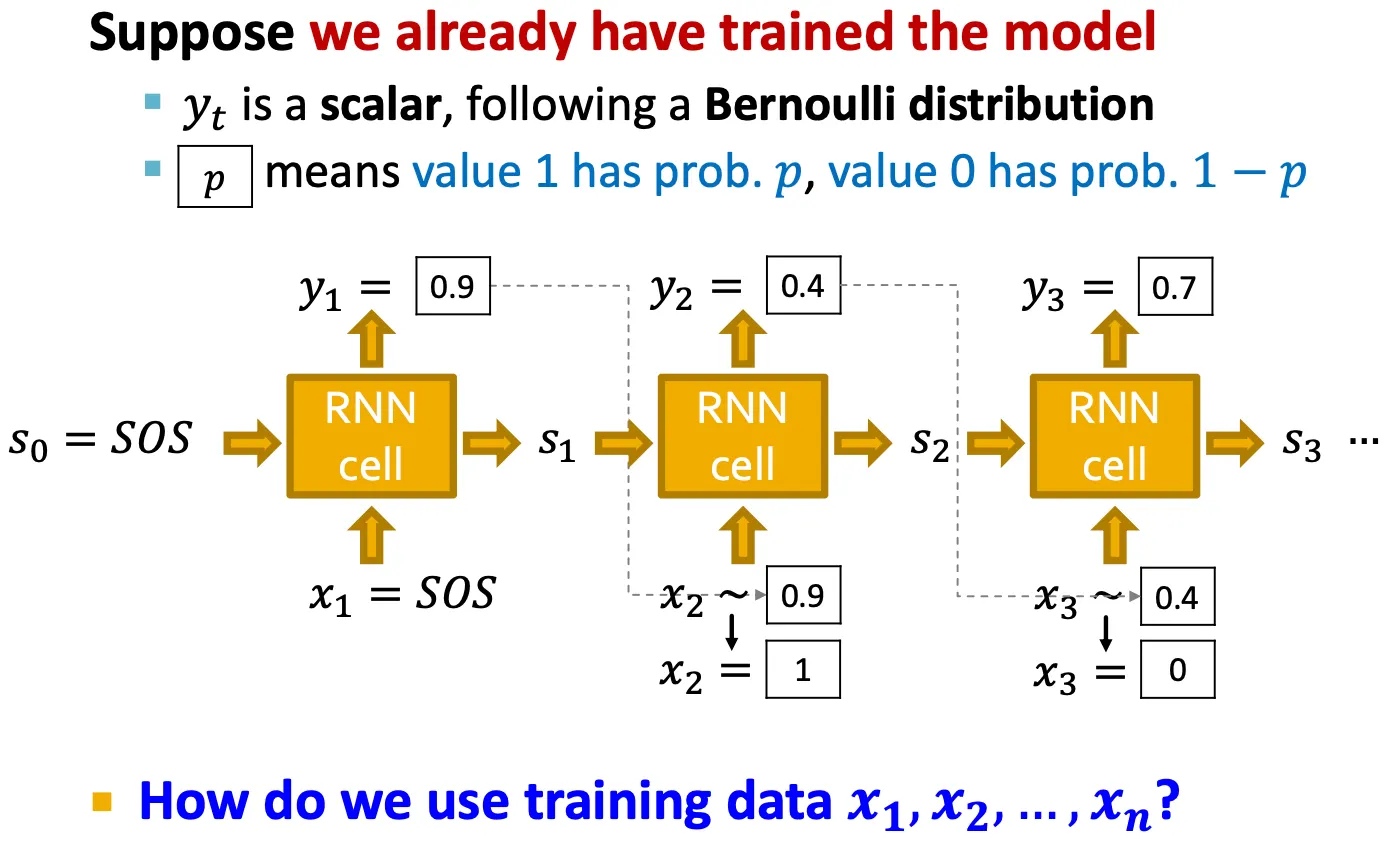
Time step 에서 를 예측하고, Bernoulli distribution에 따라 을 에서 sampling 해서 0 또는 1을 예측한다.
그 예측된 값을 그 다음 cell의 input으로 사용한다.
◦
Training time strategy
Training 시에는 edge들의 를 알 수 있으므로, 와 예측된 의 차를 loss로 계산한다.
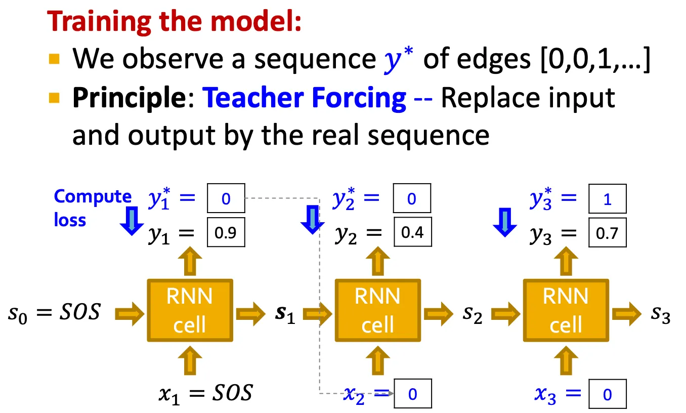
즉, teacher forcing으로, 알고 있는 를 그 다음 step의 input 로 직접 사용한다.
Loss는 binary cross entropy를 사용한다.
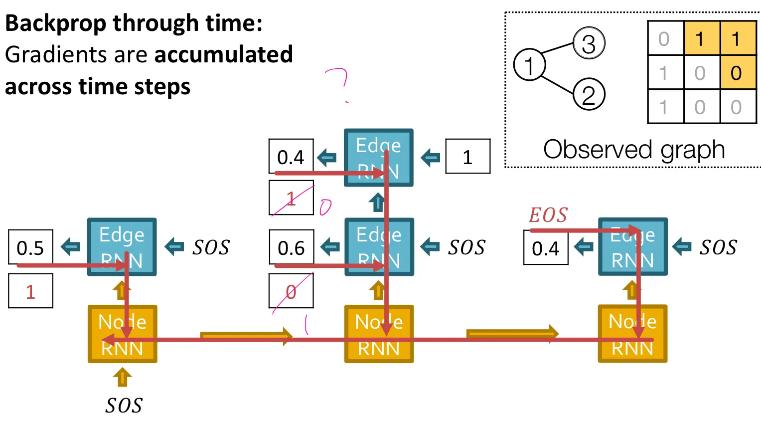
Putting things together

•
Training 시
•
Test 시
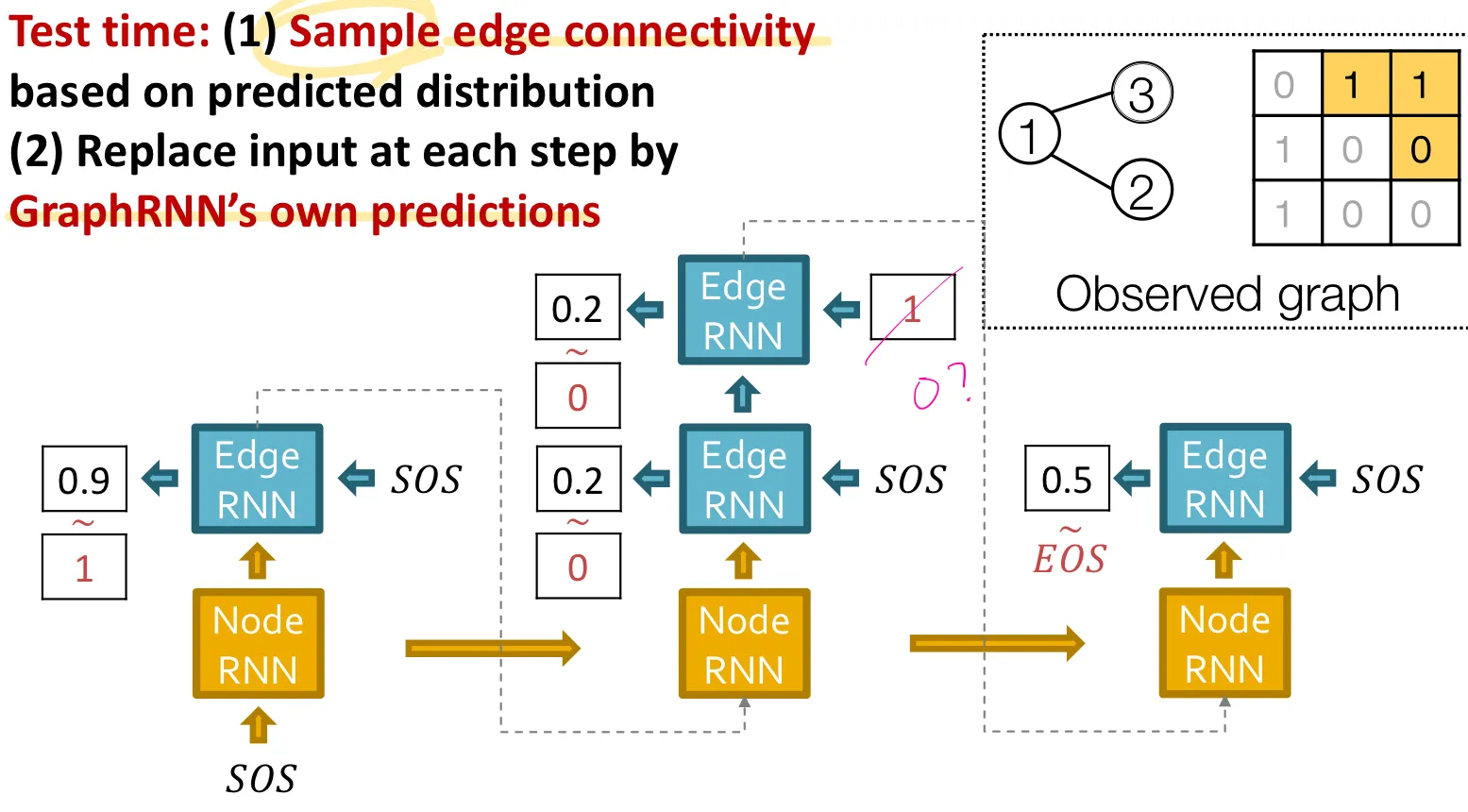
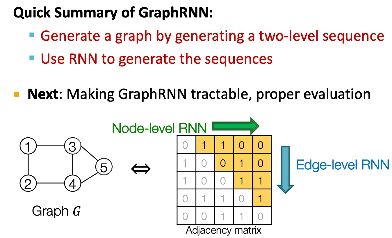
GraphRNN: Summary
•
GraphRNN은 RNN을 사용해 two-level sequence로 graph를 생성한다.
•
이제 GraphRNN을 tractable하고 성능을 잘 평가하는 방법을 다룬다.
Scaling Up and Evaluating Graph Generation
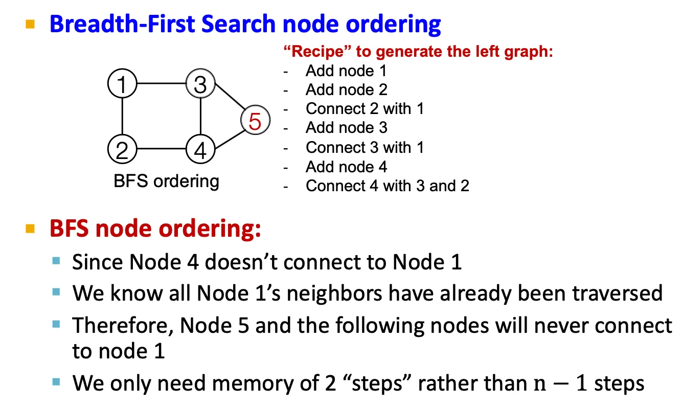
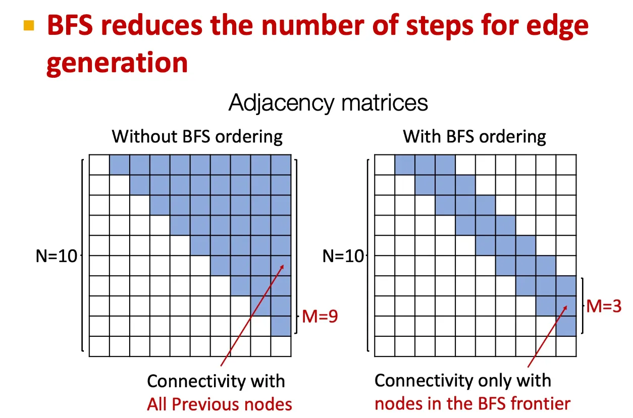
Tractability issue
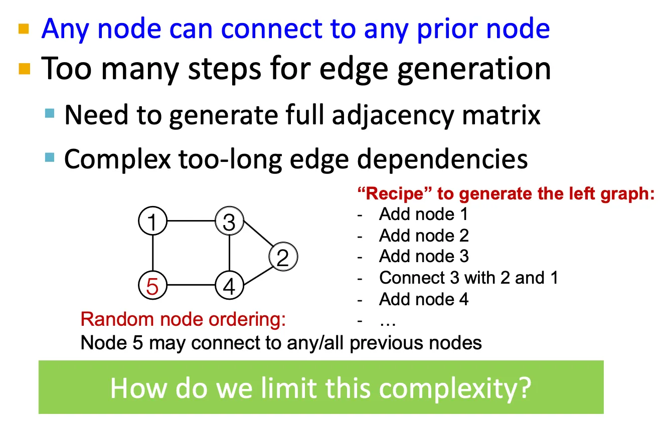
어떤 node가 이전에 존재하던 node들과 연결될 수 있을지를 모두 계산해야 하므로 intractable 하다. → BFS node ordering으로 이를 일부 해결할 수 있다.
Evaluating generated graphs
•
Graph의 집합(set)을 비교하는 방법 → graph의 similarity metric을 정의해야 한다.
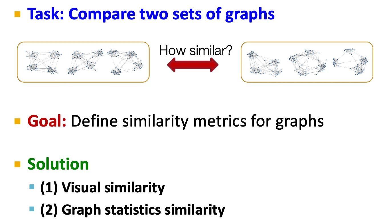
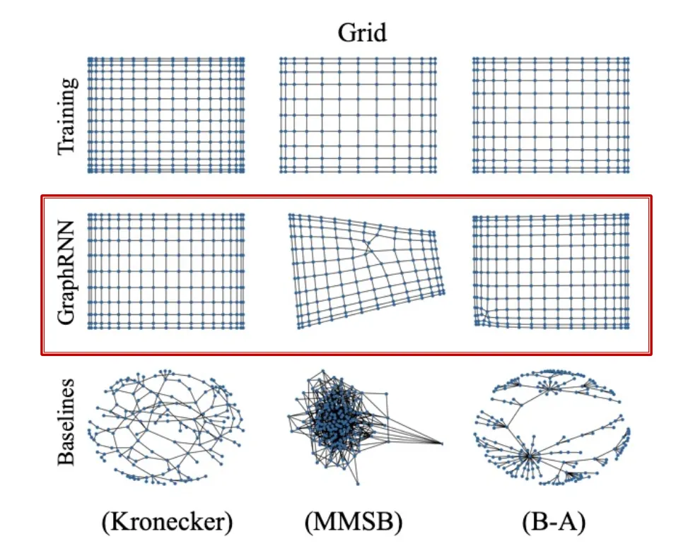
1.
Visual similarity
2.
Graph statistics similarity
직접 두 graph를 비교하는 isomorphism test는 NP!
→ Graph statistics를 비교한다.
Degree distribution, clustering coefficient distribution, orbit count statistics, … → 모두 일종의 distribution 이다.
Step 1: 두 graph statistics를 비교하는 방법
EMD (Earth Mover Distance)

Step 2: Graph statistics의 set을 비교하는 방법
MMD (Maximum Mean Discrepancy)

Application of Deep Graph Generative Models to Molecule Generation
Application: Drug discovery

•
말이 되고, 실제로 존재할만한 molecule이 어떤 property score를 만족하도록 만들 수 있을까?
1.
High score: 어떤 objective에 대해 optimize
e.g.) drug-likeness
→ RL을 이용
2.
Valid: 특정 rule을 반드시 만족하도록
e.g.) Chemical validaty rule
3.
Realistic: 실제 example로부터 학습
e.g.) Molecule graph dataset
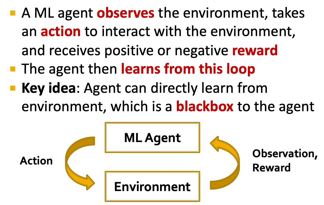
Idea: Reinforcement Learning
•
ML agent가 environment를 관찰하고, 어떤 action을 취해 reward를 얻는 것.
GCPN: Graph Convolutional Policy Network
•
Key component
◦
GNN: graph의 structural info capture
◦
RL: 원하는 objective를 얻도록 generation guide
◦
Supervised training: 주어진 dataset의 example을 imitate
•
GCPN vs GraphRNN
공통점
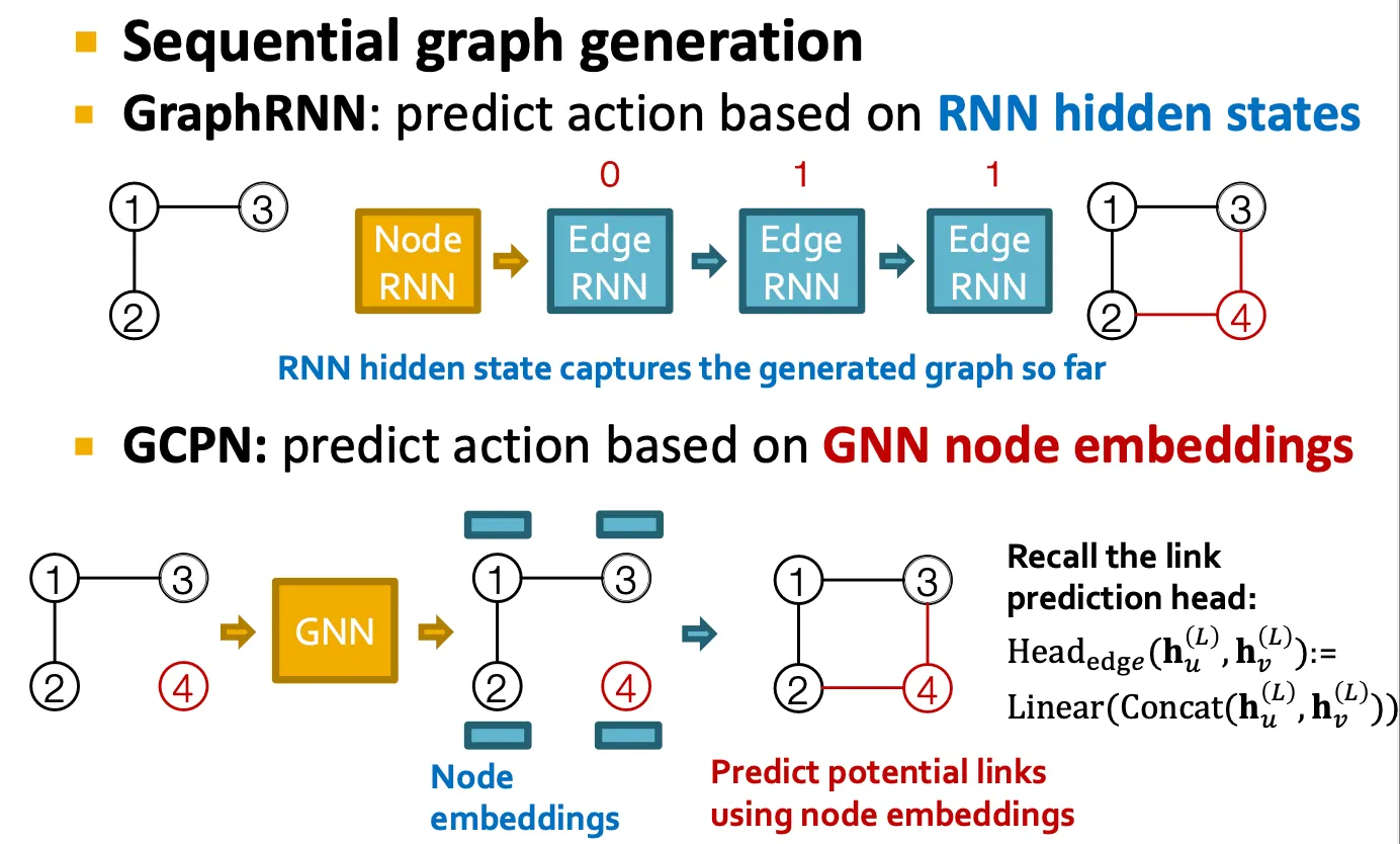
◦
Graph를 순차적으로 generate
◦
주어진 graph dataset을 imitate
차이점
◦
GCPN은 RNN이 아닌 GNN을 사용해 generation action을 예측
◦
GCPN은 RL을 이용해 graph generation을 guide
Overview of GCPN
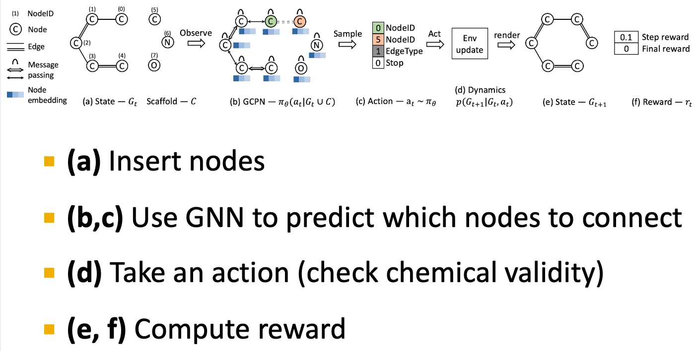
•
Reward 설정
◦
Step reward: valid action을 선택하도록, small reward를 설정한다.
◦
Final reward: desired property를 optimize 하도록 big reward를 설정한다.
Training GCPN: Two parts
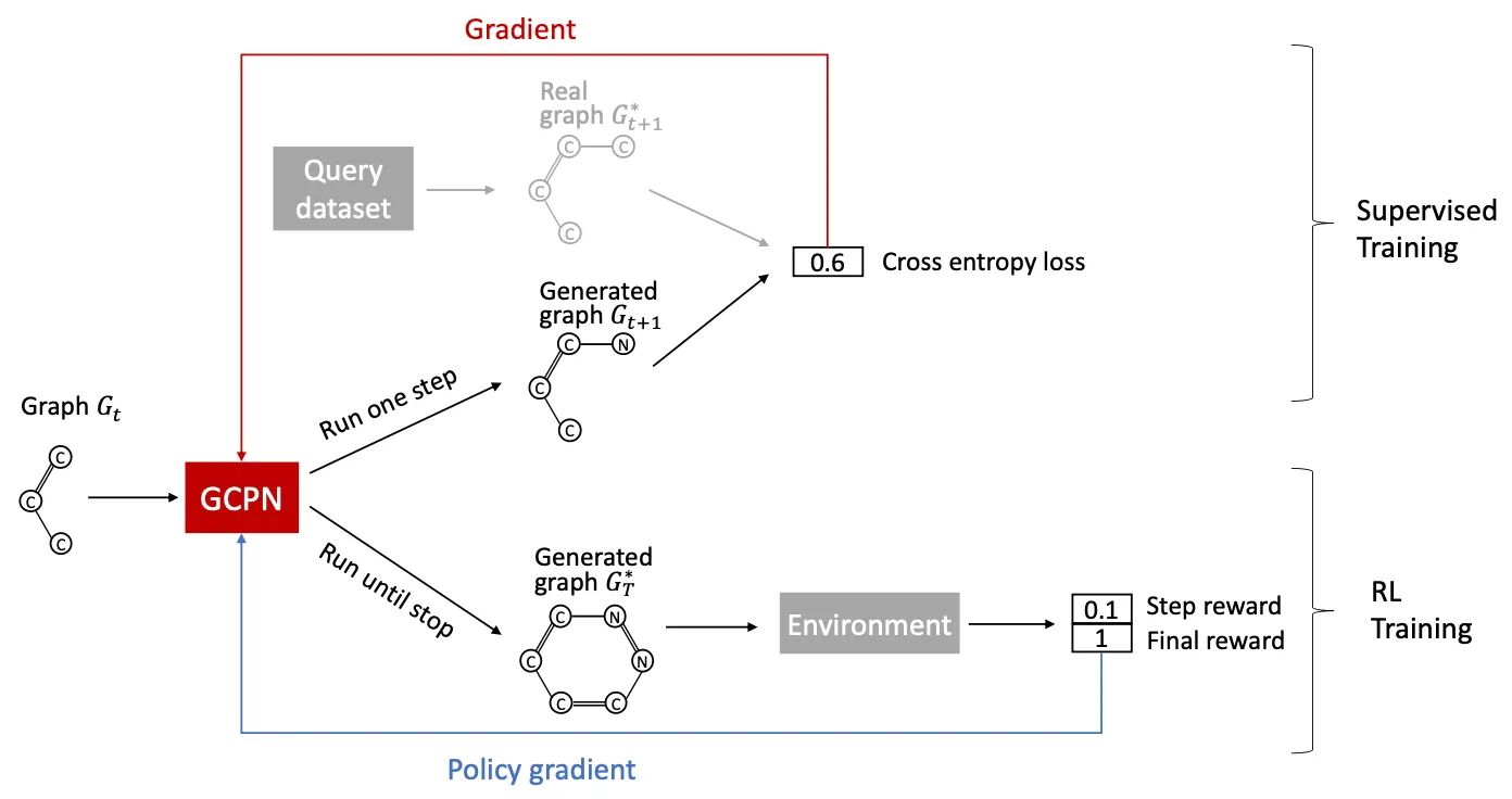
1.
Supervised training
Real observed graph에서 얻은 action을 imitate하도록 policy를 학습.
Gradient-based training.
2.
RL training
Reward optimization.
Policy gradient based training.