

8.1 Graph Augmentation
8.2 Prediction with GNNs
8.3 Training Graph Neural Networks
8.4 Setting-up GNN Prediction Tasks
8.1 Graph Augmentation
•
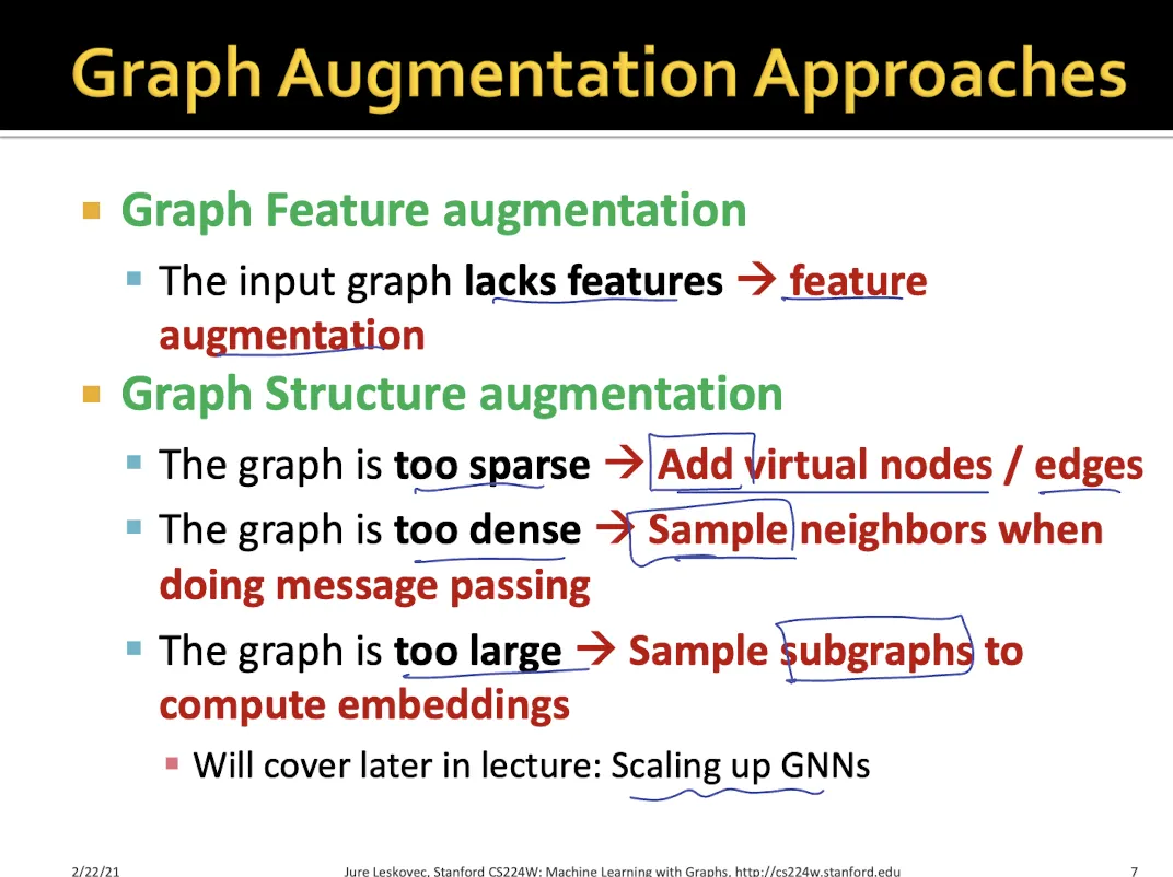
raw input graph를 그대로 GNN 계산하는데 사용하면 여러가지 문제가 있을 수 있다.
•
Feature Augmentation을 하는 이유
◦
input graph의 feature들이 부족해서 graph의 특징을 제대로 표현하지 못하는 경우
•
Structure Augmentaion을 하는 이유
◦
graph가 너무 sparse할 때 → 각 node 정보가 잘 전달되지 않을 수 있음 → Add virtual nodes or edges
◦
너무 dense 할 때 → high computational cost and overfitting→ sample neighbors while aggregating
◦
graph가 너무 클 때 → high computational cost → subgraph
Feature Augmentation
1.
Input graph에 node feature가 없을 때
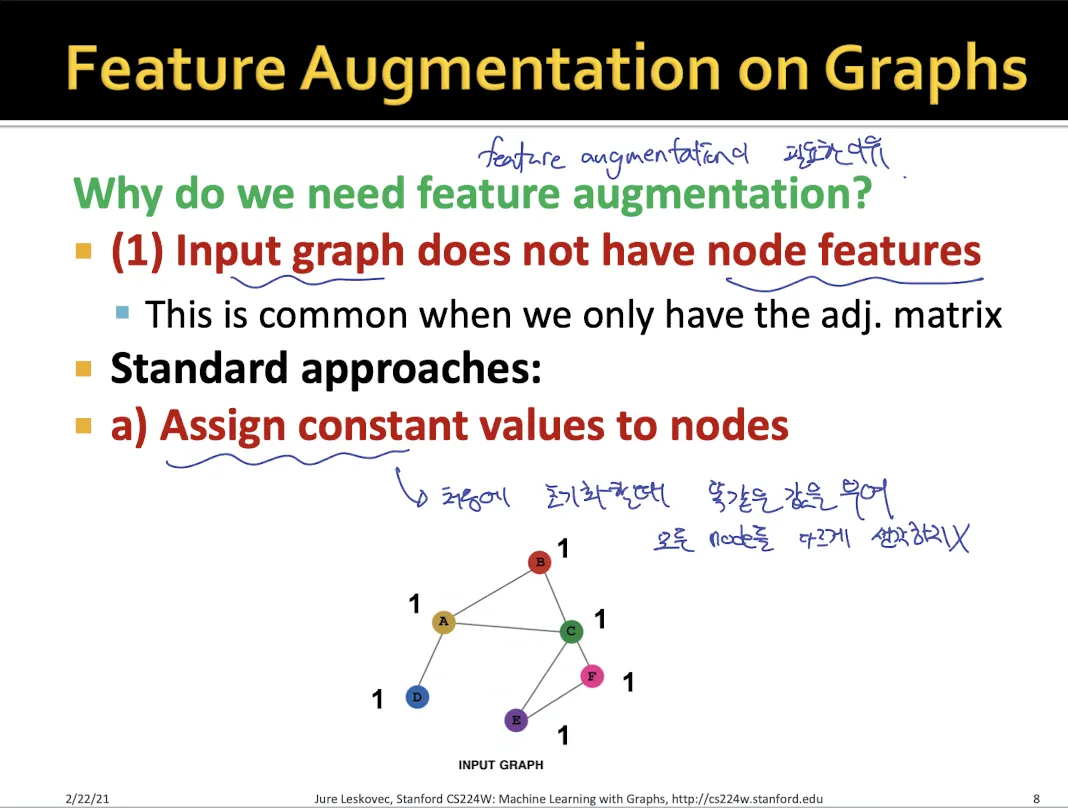
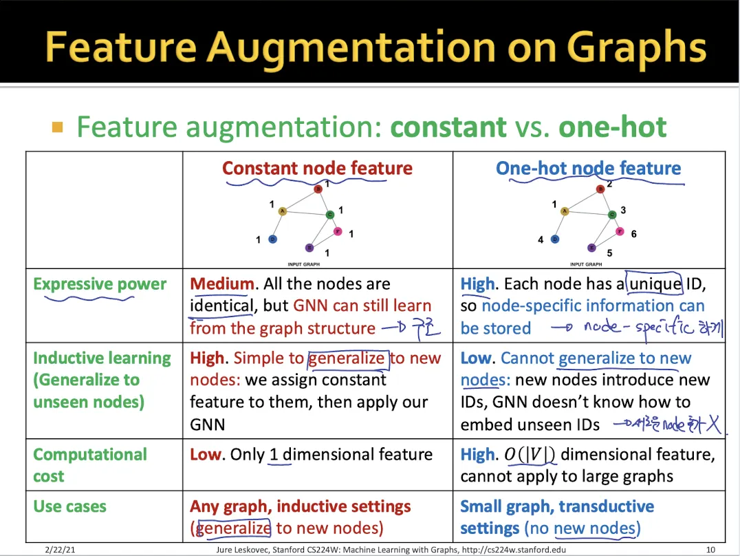
a.
Constant node feature
•
모든 node에 대해서 동일한 feature 값을 부여한다. (1-dimensional feature)
•
graph structure를 알 수 있다는 장점이 있다.
•
새로운 node가 들어왔을 때 추가하기 쉽다.
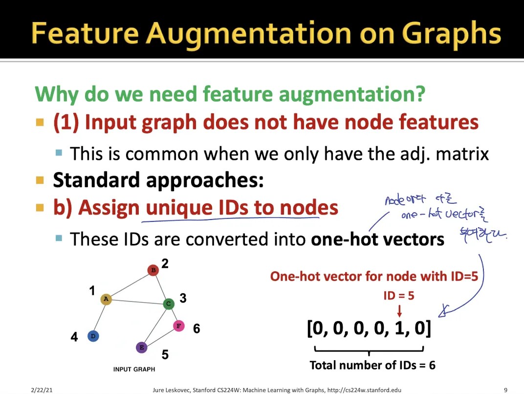
b.
One-hot node feature
•
각각의 node는 독립적으로 생각하여 고유의 아이디를 부여
•
node-specific한 feature 정보를 담을 수 있다.
•
새로운 node를 추가하기는 어렵다
•
high computational cost
2.
graph structure와 같이 GNN으로는 알기 힘든 정보들이 있을 때
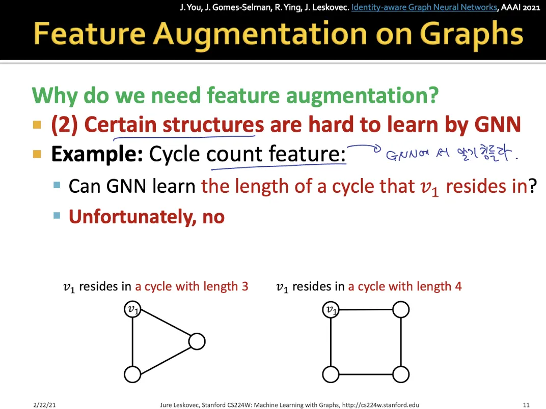
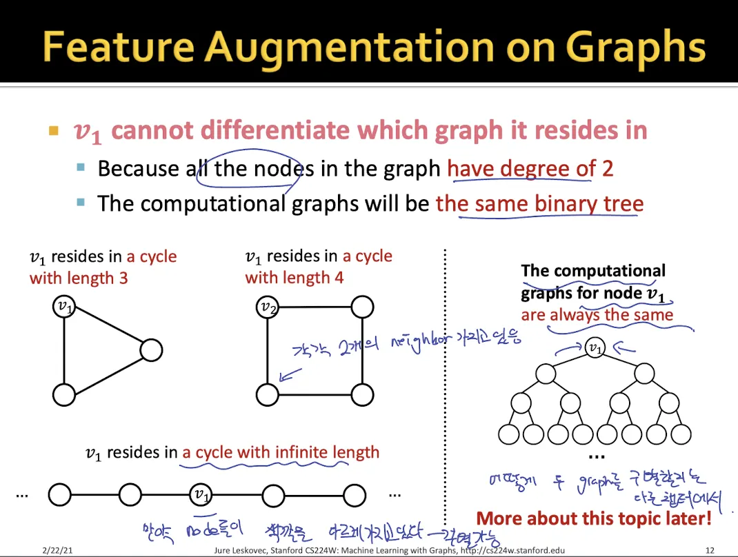
•
위와 같이 삼각형, 사각형 graph가 있을 때 모든 node들은 degree 2를 가지기 때문에 GNN으로 두 graph를 구별할 수가 없다.
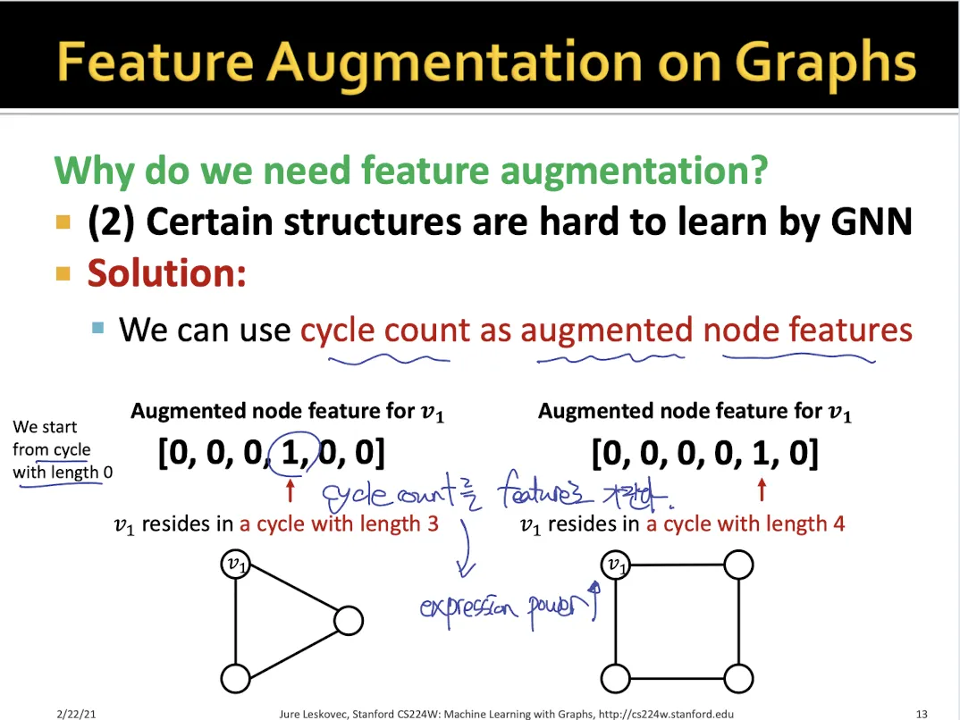
•
각 node가 어떤 cycle에 해당되는지를 feature로 만든다.
•
만약 3 cycle과 4 cycle 둘다 속한다면 → [0, 0, 0, 1, 1, 0]
•
cycle 수를 통해서 두 graph의 node들을 구별할 수 있고, 두 graph의 구조가 다른 것을 알 수 있다.
Structure Augmentaion
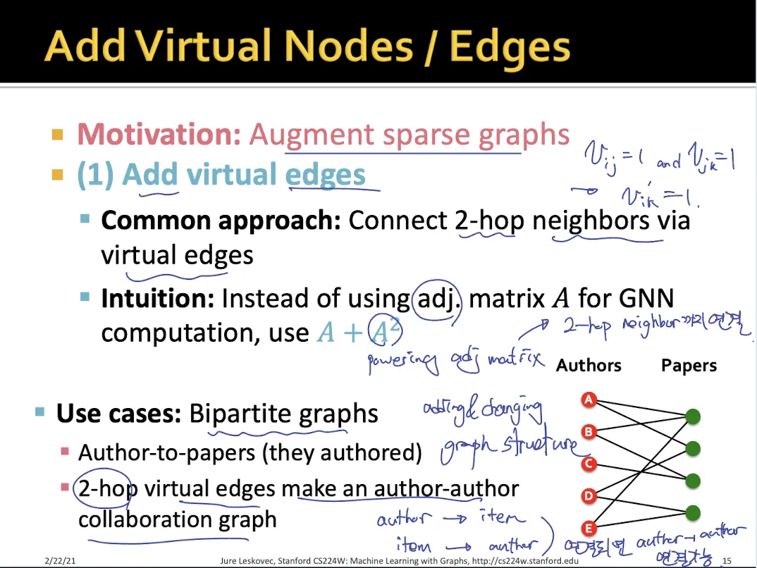
1.
Add virtual edges
•
sparse graph의 경우 사용한다.
•
A+A^2 matrix를 사용한다.
•
2-hop neighbor끼리도 edge로 연결된다.
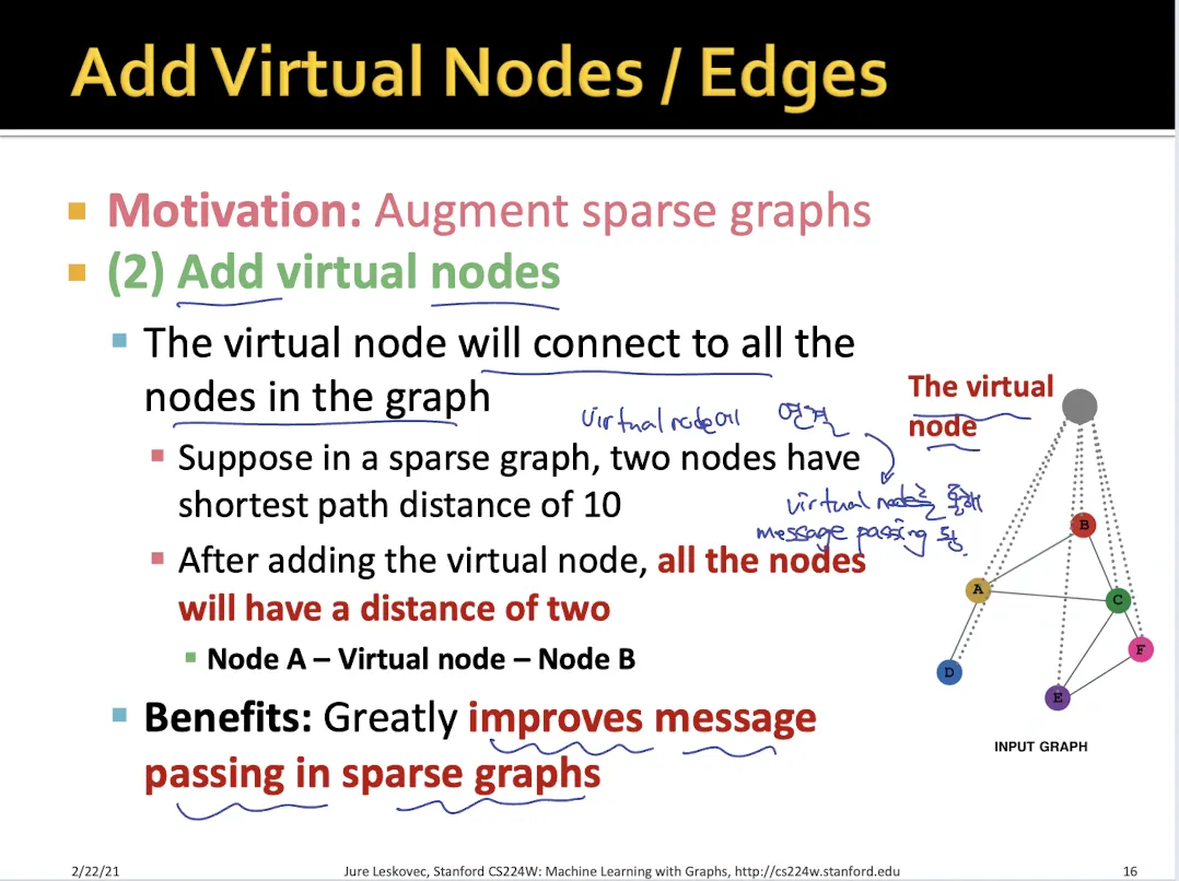
2.
Add virtual nodes
•
모든 node들이 연결되어 있는 virtual node를 만든다.
•
virtual node를 통해서 원래는 멀리 떨어져 있던 node 한테도 message passing이 이뤄진다.
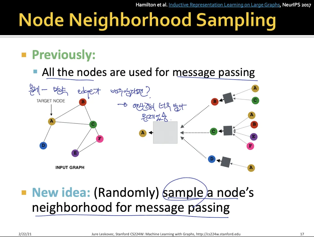
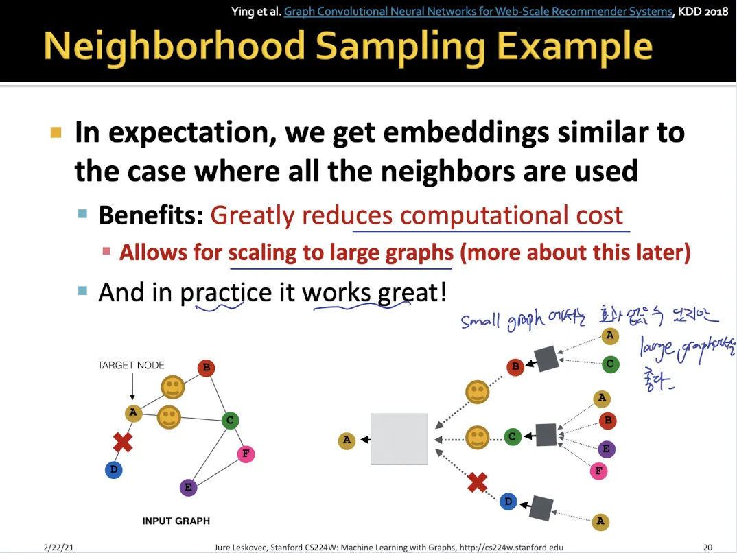
3.
Sampling
•
dense한 graph에서 사용
•
모든 neighbor들을 message passing에 사용하지 않고 일부만 sampling하여 사용한다.
•
dropout와 같은 효과
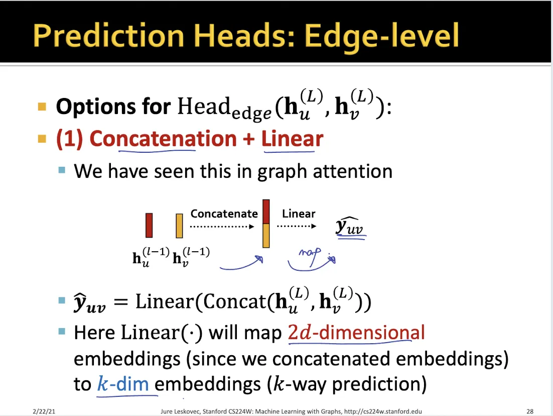
8.2 Prediction with GNNs
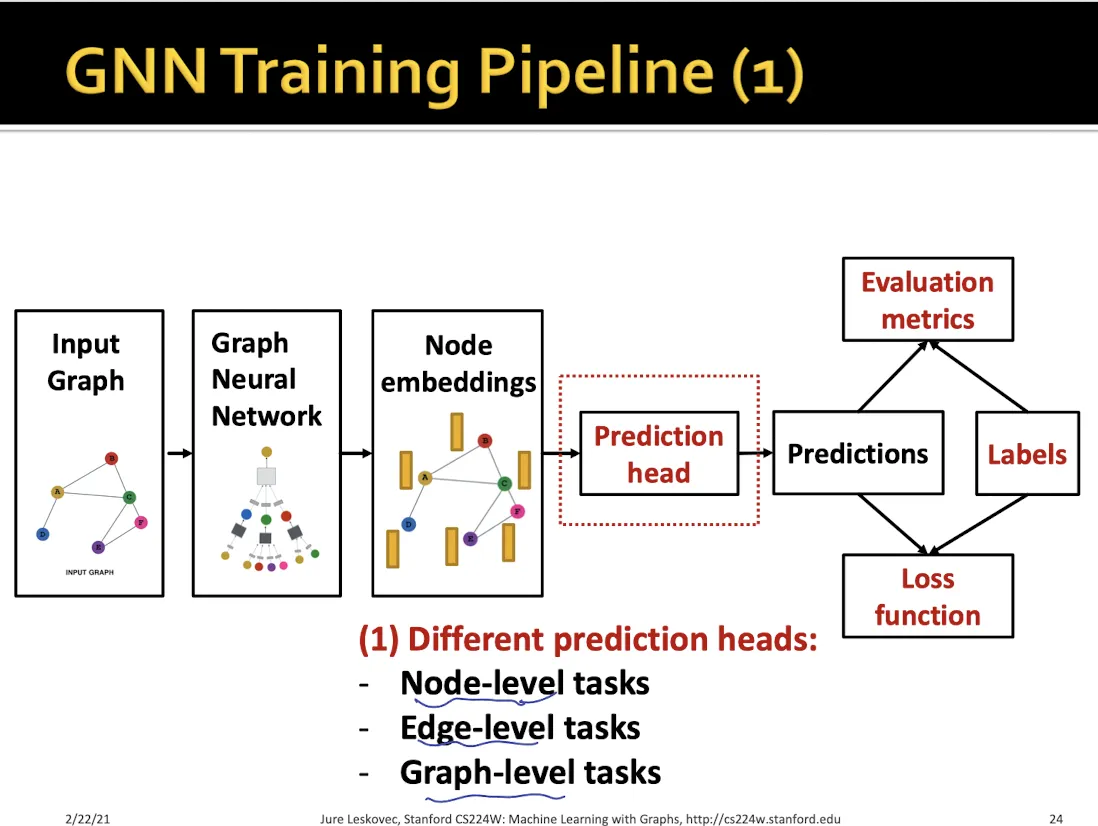
Prediction Head
1.
Node-level prediction
2.
Edge-level prediction
3.
Graph-level prediction
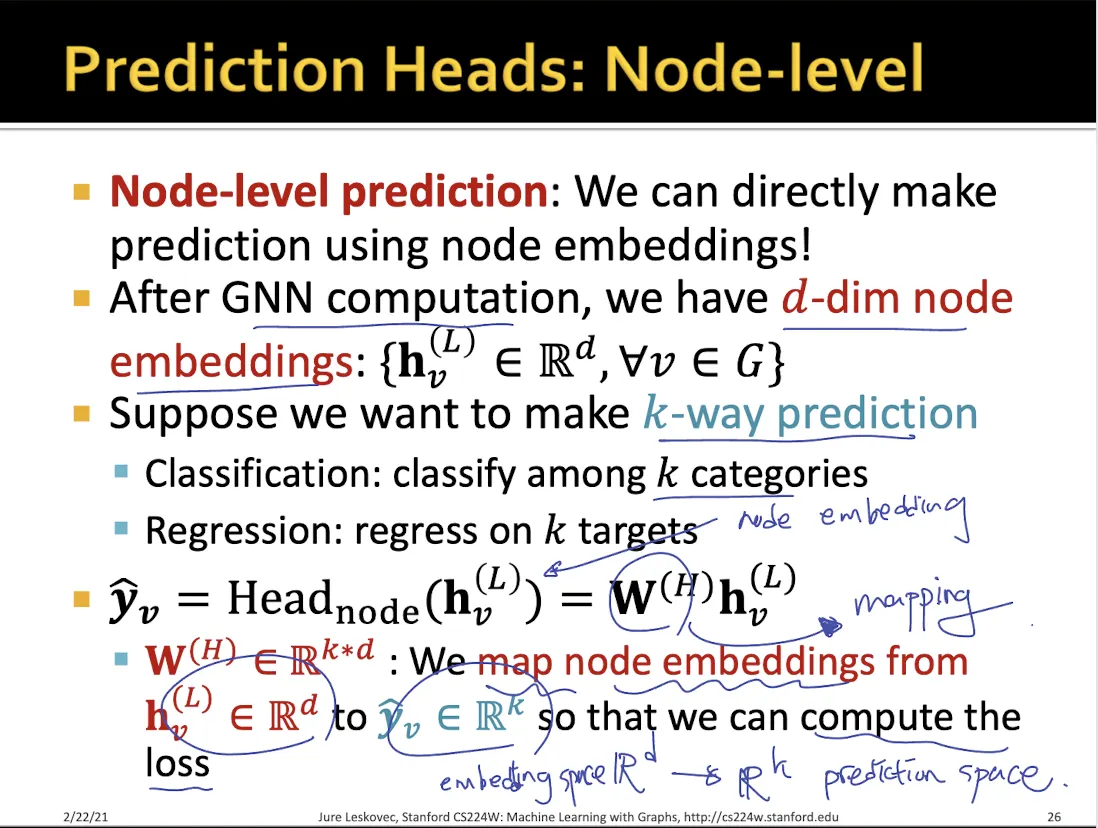
•
Node level prediction
•
node embedding을 prediction space로 mapping하여 사용한다.
•
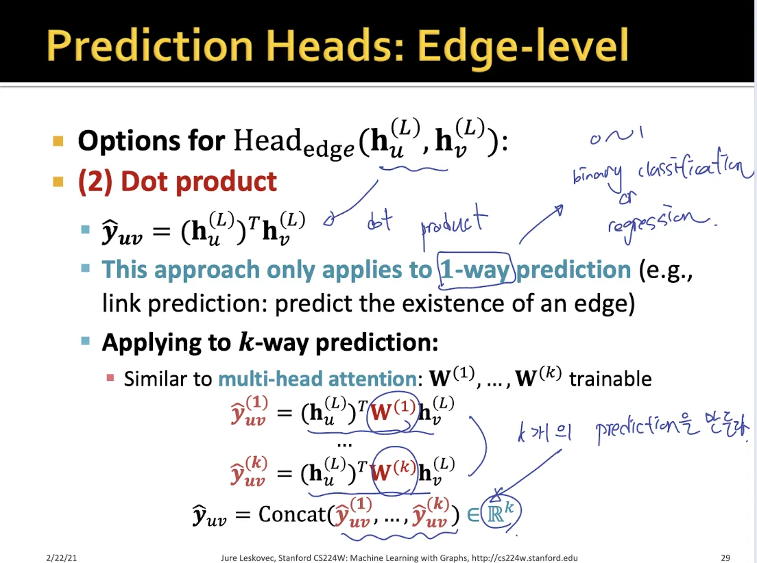
Edge level prediction
•
concate 후 mapping하는 방식
•
dot product 하는 방식
◦
dot product 할 때 중간에 matrix를 추가로 두어 mapping하면 multi classification도 가능하다.
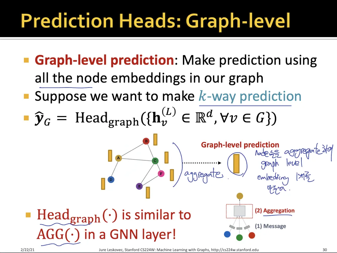
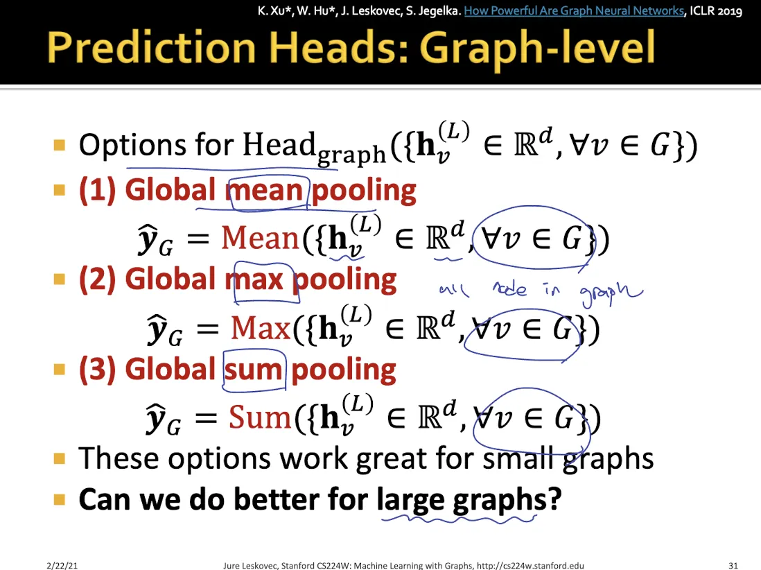
•
Global level prediction
•
graph에 있는 모든 node들의 feature들을 합치는 여러가지 방법이 있다. (mean, max, sum …)
•
하지만 이런 global pooling으로는 graph에 있는 정보가 많이 손실된다는 단점이 있다.
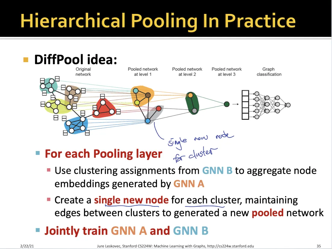
•
위의 문제를 해결하기 위해 나온 것이 DiffPool
•
sub graph cluster에서 pooling을 하고, 그렇게 나온 node들을 다시 pooling하여 global embedding을 만들어낸다.
8.3 Training Graph Neural Networks
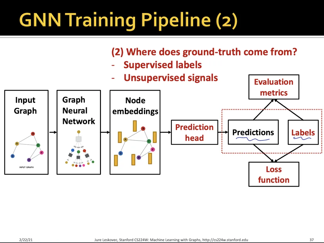
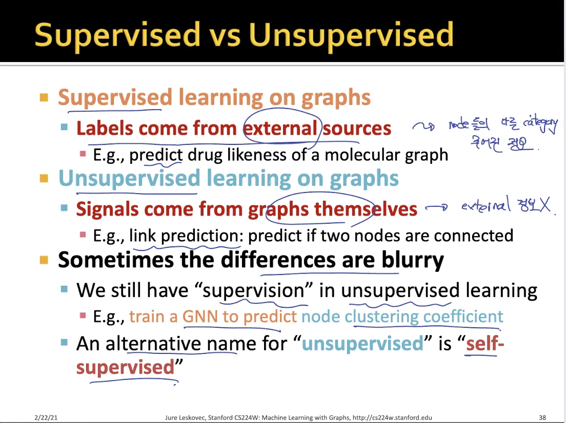
Supervised learning, unsupervised learning으로 나눌 수 있다.
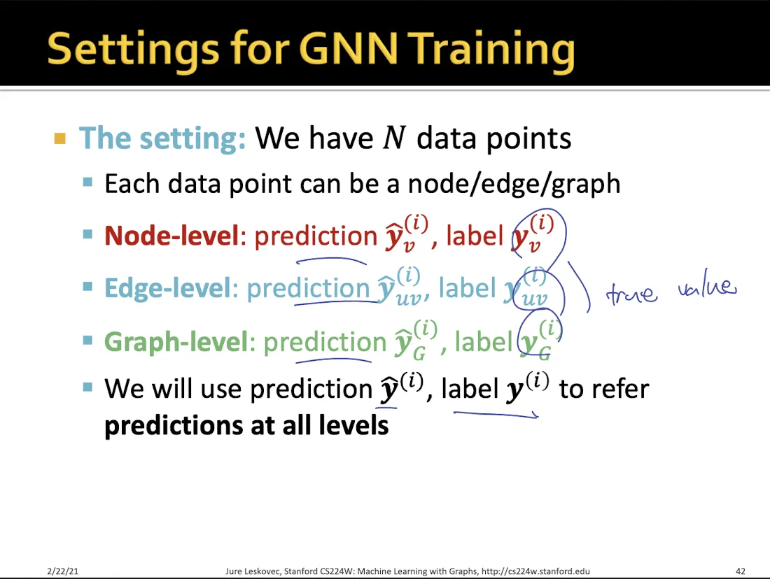
•
Supervised training의 경우 node/edge/graph 마다 true value가 있어서 prediction 에 대해서 loss를 계산한다.
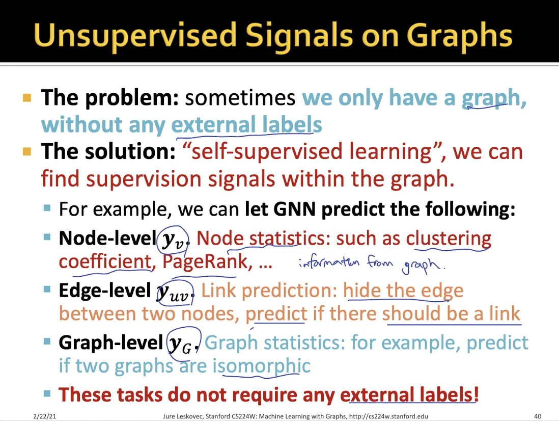
•
Unsupervised training은 external label이 없다.
•
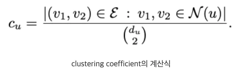
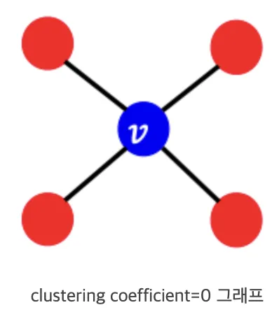
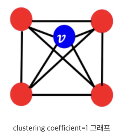
node-level에 대해서는 clustering coefficient, pagerank등을 맞춘다.
◦
clustering coefficient 은 neighbor node끼리 얼마나 잘 이어져 있는지 나타내는 정도
•
edge-level에 대해서는 edge를 일부러 없앤다음 link가 있는지 맞춘다.
•
graph-level에 대해서는 두 그래프가 isomorphic한지 맞춘다.
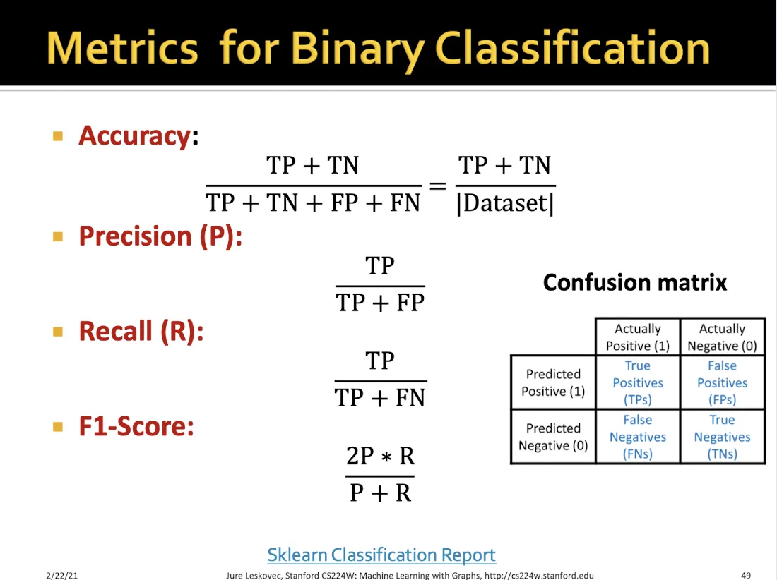
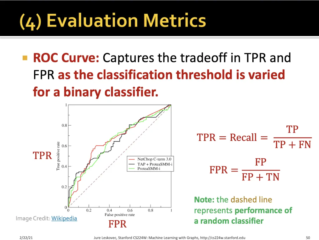
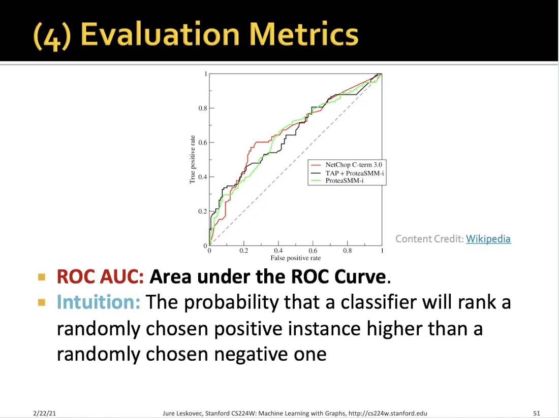
Metrics
8.4 Setting-up GNN Prediction Tasks
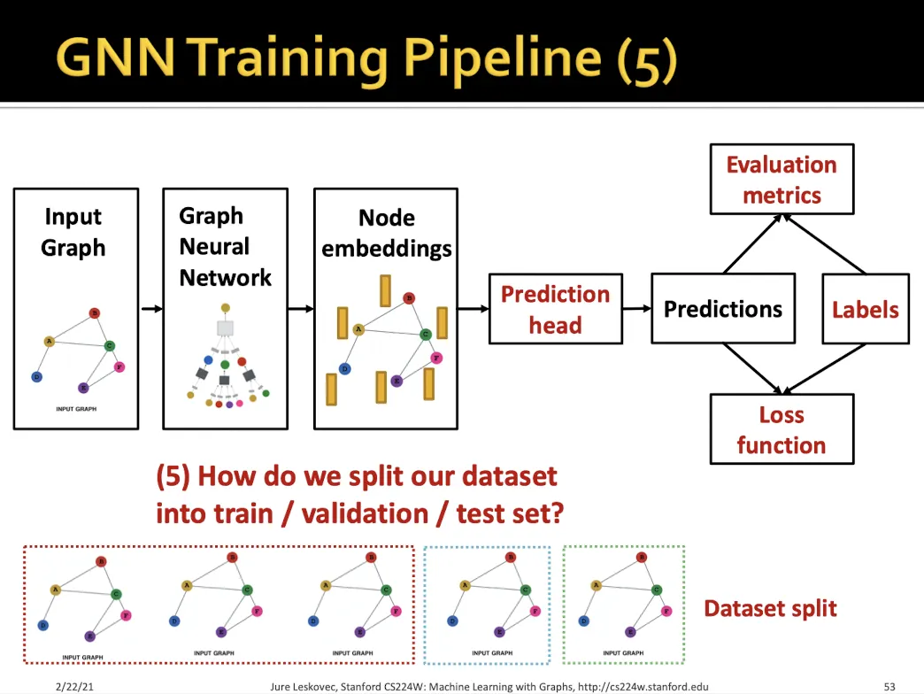

Train, valid, test를 나누는 방법
1.
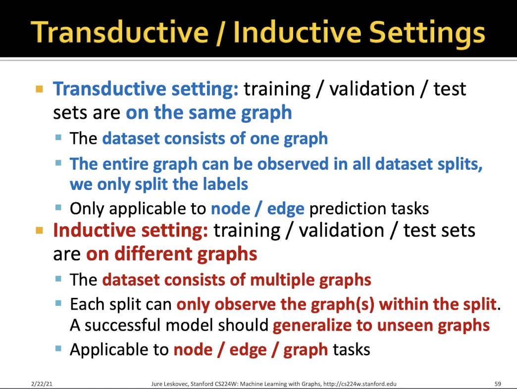
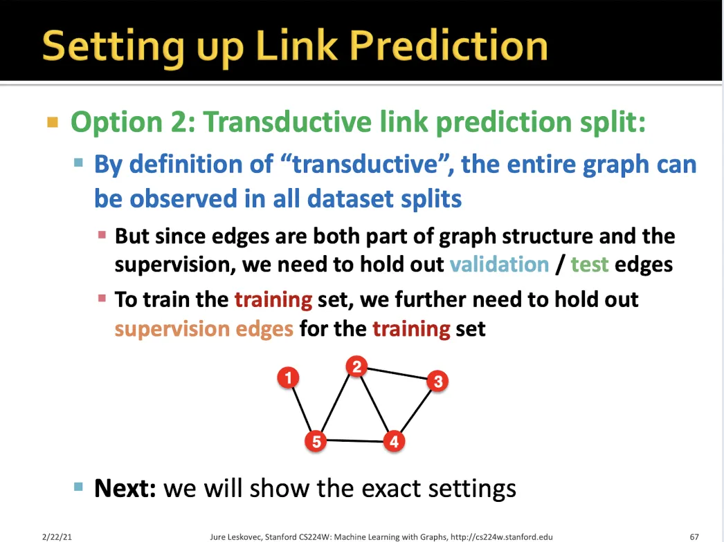
Transductive setting
•
그래프 전체를 사용하되 일부 라벨만 train/valid/test 로 나눠서 학습에 사용한다.
•
하나의 그래프 사용
2.
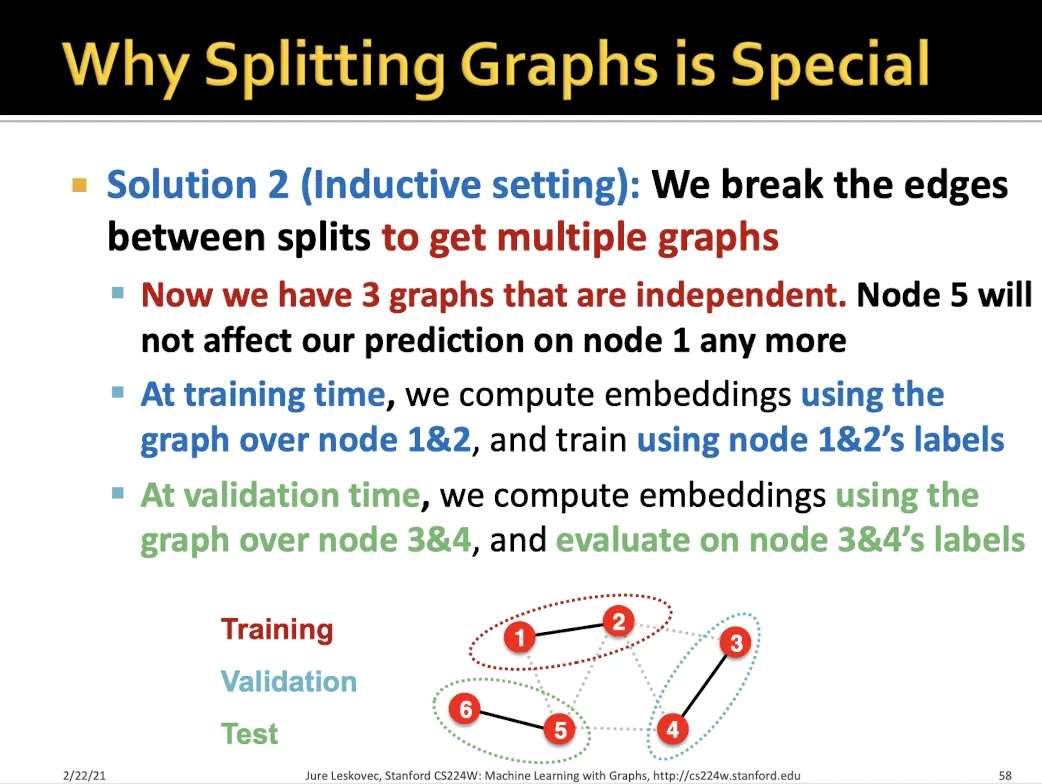
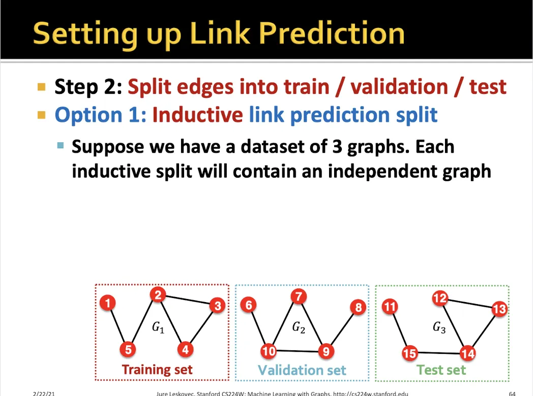
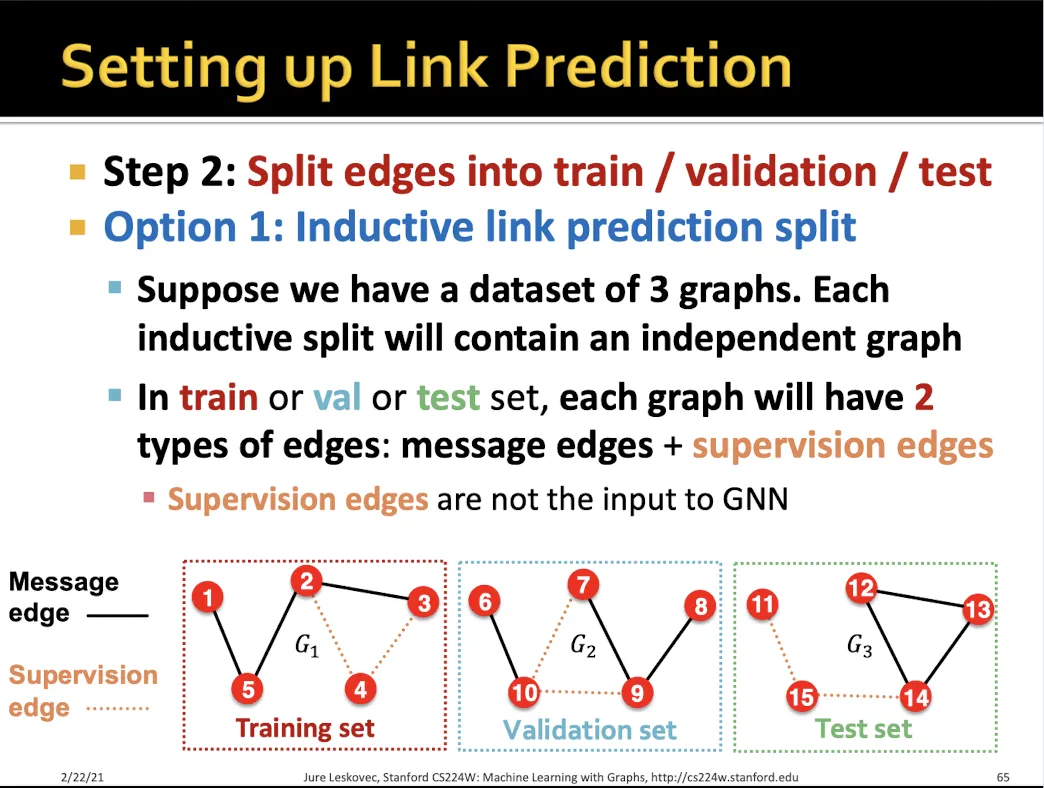
Inductive setting
•
edge를 잘라서 여러개의 그래프로 만든다.
•
각각의 graph에 대해서 학습을 진행한다.
•
여러개의 그래프 사용
•
unseen graph에 대한 generalization도 가능하다
여러가지 Tasks에 대한 split setting
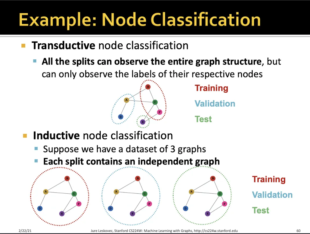
Node classification
•
Transductive → node를 train/valid/test에 맞게 나눠서 학습한다
•
Inductive → 하나의 그래프에서 node들을 drop 시켜서 여러개의 독립적인 그래프를 만들어 진행한다
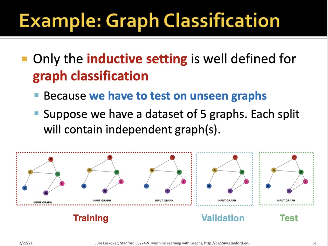
Graph classification
•
Transductive → 불가능
•
Inductive → 각각을 독립적인 그래프라 생각하고 분류 학습
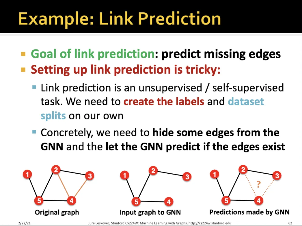
Link prediction
•
Transductive, Inductive 둘다 가능하다
•
Inductive로 link prediction 하는 방법?
•
마찬가지로 edge를 없애서 여러개의 graph를 만든다.
•
각각의 graph에서 message edge, supervision edge를 만든다.
•
message edge는 학습에 사용되고, supervision은 message passing에 사용되지 않는다.
•
각 graph에서 supervision edge의 link를 맞추는 것이 목표이다.
•
Transductive link prediction 하는 방법?
•
하나의 graph에서 edge들을 여러가지 종류로 나눈다.
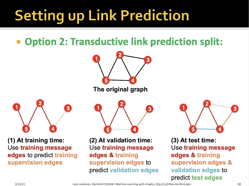
•
Training에서는 training message edge로 학습하여 training supervision edge를 맞춘다.
•
Validation에서는 training message edge + training supervision edge로 학습하여 validation edge를 맞춘다.
•
Test에서는 test edge를 맞춘다.
→ Traning message, training supervision, validation edge, test edge 총 4가지로 나눈다.
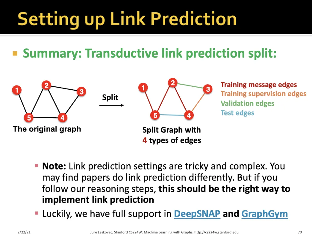
•
단점 : 복잡하다