

.png&blockId=184de6ac-9693-4d9d-880f-7ce9c450c1ca&width=3600)

Summary
•
Few shot learning을 위해 다른 sample과의 similarity 정보까지 이용(즉, 각 sample의 label을 독립적으로 학습하는데서 그치지 않음)
•
각 sample을 graph의 node라고 보고, edge는 두 sample간의 similarity kernel로 간주.
•
Edge, 즉 similarity kernel은 trainable 함(즉, 단순한 inner product 등으로 pre-defined 되지 않음)
•
Node의 feature는 message passing algorithm에서 착안하여 각 time step 마다 이웃 node에서 message를 받아서 업데이트됨.
•
Semi-supervised learning, 더 나아가 active learning에도 적용 가능.
•
Omniglot, Mini-ImageNet에 대해 더 적은 parameter로 state-of-the-art 성능을 보여줌(2017년 기준)
Keywords
•
Few shot learning
•
Graph neural network
•
Semi-supervised learning
•
Active learning with Attention
1. Introduction
•
Supervised end-to-end learning has been extremely successful in computer vision, speech, or machine translation tasks.
•
However, there are some tasks(e.g. few shot learning) that cannot achieve high performance with conventional methods.
•
New supervised learning setup
◦
Input-output setup:
▪
With i.i.d. samples of collections of images and their associated label similarity
▪
cf) conventional setup: i.i.d. samples of images and their associated labels
•
Authors' model can be extended to semi-supervised and active learning
◦
Semi-supervised learning:
Learning from a mixture of labeled and unlabeled examples
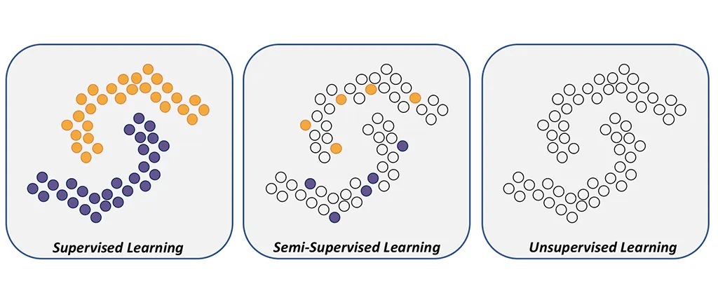
◦
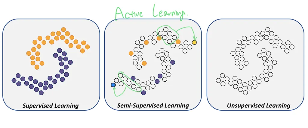
Active learning:
The learner has the option to request those missing labels that will be most helpful for the prediction task
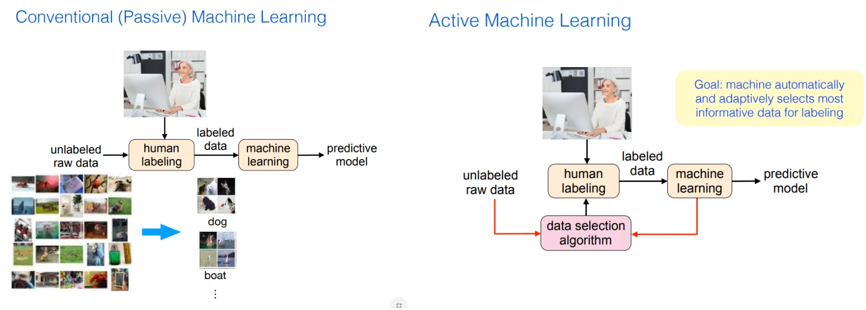
ICML 2019 active learning tutorial
Annotated by JH Gu
2. Closely related works and ideas
[Research article] Matching Networks for One shot learning - Vinyals et al.(2016)
[Research article] Prototypical Networks for Few-shot Learning - Snell et al.(2017)
[Review article] Geometric deep learning - Bronstein et al.(2017)
[Research article] Message passing - Gilmer et al.(2017)
3. Problem set-up
Authors view the task as a supervised interpolation problem on a graph
•
Nodes: Images
•
Edges: Similarity kernels → TRAINABLE
General set-up
Input-output pairs drawn from i.i.d. from a distribution of partially labeled image collections
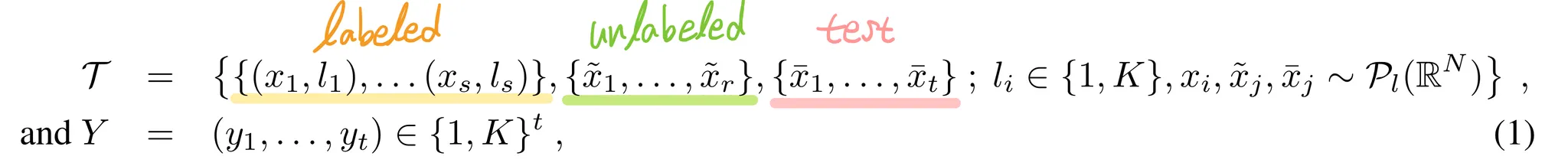
•
: # labeled samples
•
: # unlabled samples
•
: # samples to classify
•
: # classes
•
: class-specific image distribution over
•
targets are associated with
Learning objective:
( is the standard regularization objective)
Few shot learning setting
Semi-supervised learning setting
Model can use the auxiliary images(unlabeled set) to improve the prediction accuracy, by leveraging the fact that these samples are drawn from the common distributions.
Active learning setting
The learner has the ability to request labels from the auxiliary images .
4. Model
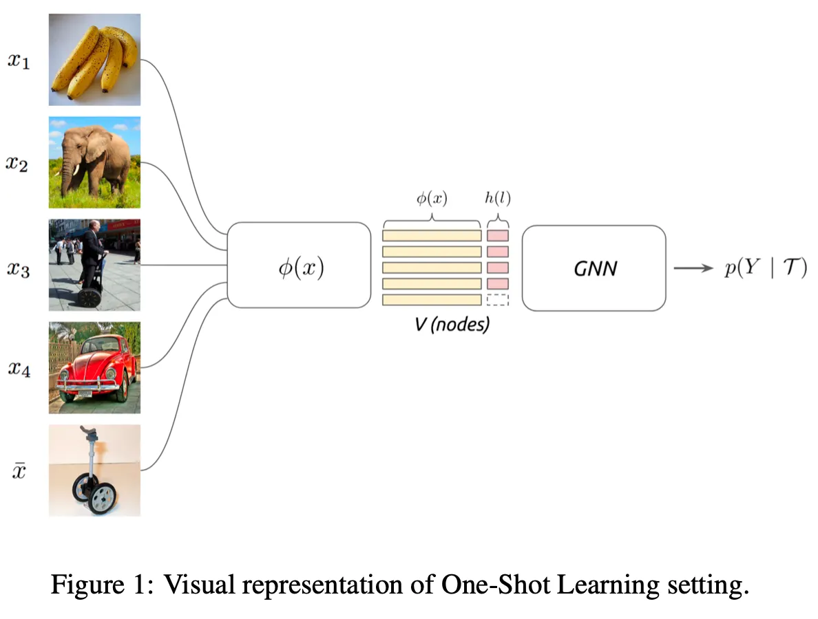
•
: CNN
•
: One-hot encoded label(for labeled set), or uniform distribution(for unlabeled set)
4.1. Set and Graph Input Representations
The goal of few shot learning:
To propagate label information from labeled samples towards the unlabeled query image
→ The propagation can be formalized as a posterior inference over a graphical model
Similarity measure is not pre-specified, but learned!
c.f.) in Siamese network, the similarity measure is fixed(L1 distance)!
본 논문(Few shot learning with GNN)에 쓰인 문장 구조가 이상해서 헷갈리게 쓰여있음.
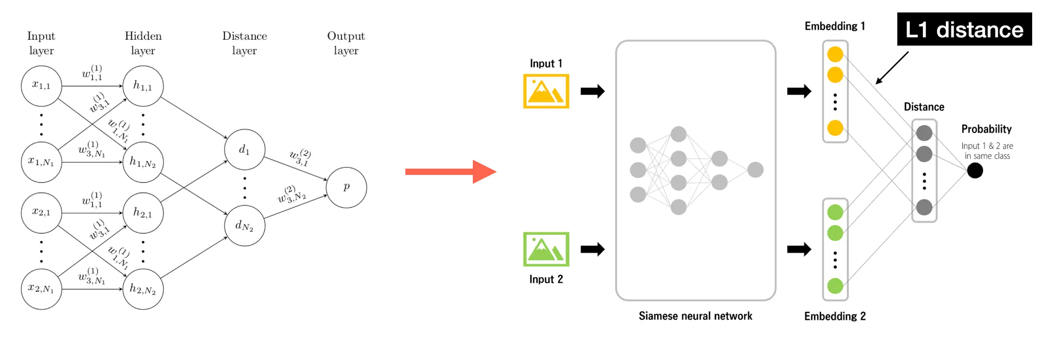
Koch et al.(2015), https://tyami.github.io/deep learning/Siamese-neural-networks/
4.2. Graph Neural Networks
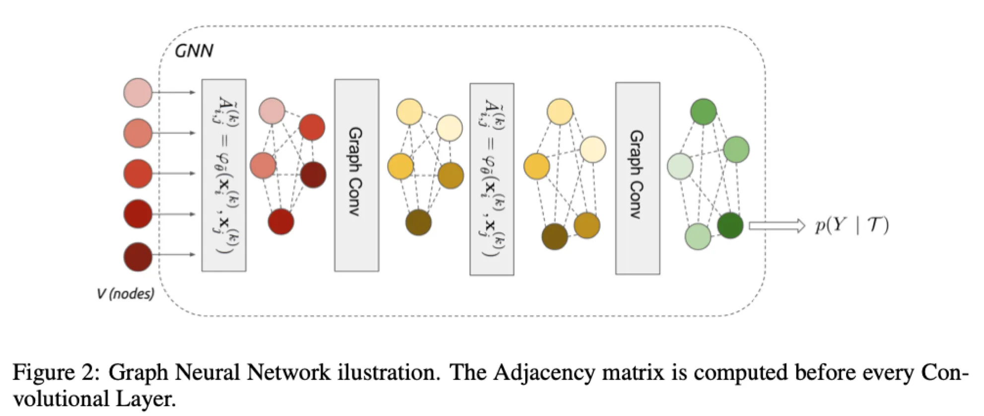
We are given an input signal on the vertices of a weighted graph .
Then we consider a family, or a set "" of graph intrinsic linear operators.
•
Linear operator
e.g.) Simplest linear operator is adjacency operator , where ( is associated weight)
GNN layer
A GNN layer receives as input a signal and produces
: representation vector of a certain node at time step
: trainable parameters
: Leaky ReLU
Construction of edge feature matrix, inspired by message passing algorithm
•
: learned edge features from the node's current hidden representation(at time step )
•
: a metric and a symmetric function parameterized with neural network
→ is then normalized by row-wise softmax
→ And added to the family
•
: Identity matrix, which is the self-edge to aggregate vertex's own features
Construction of initial node features
: convolutional neural network
: a one-hot encoding of the label
For images with unknown label, (unlabeled data) and (test data), is set with uniform distribution.
5. Training
5.1. Few-shot and Semi-supervised learning
The final layer of GNN is a softmax mapping. We then use cross-entropy loss:
The semi-supervised setting is trained identically, but the initial label fields of s will be filled with uniform distribution.
5.2. Active learning (with attention)
In active learning, the model has the intrinsic ability to query for one of the labels from .
The network will learn to ask for the most informative label to classify the sample .
The querying is done after the first layer of GNN by using a softmax attention over the unlabeled nodes of the graph.
Attention
We apply a function that maps each unlabeld vector node to a scalar value.
A softmax is applied over the scalar values obtained after applying :
: # unlabeled samples
To query only one sample we set all elements to zero except for one. →
•
At training, model randomly samples one value based on its multinomial probability.
•
At test, model just keeps the maximum value.
Then we multiply this with the label vectors
( is scaling factor)
This value is then summed to the current representation.
6. Results
6.1. Few-shot learning
Omniglot
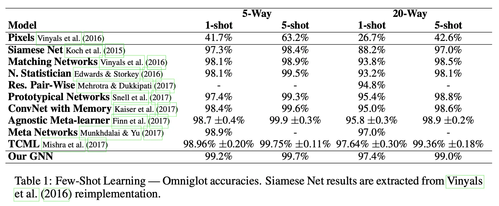
# of parameters: ,
Omniglot:
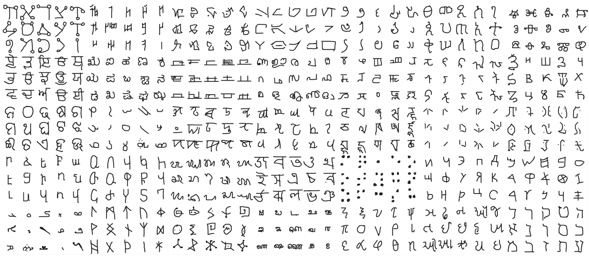
Omniglot
1,623 characters X 20 examples for each characters
Mini-ImageNet
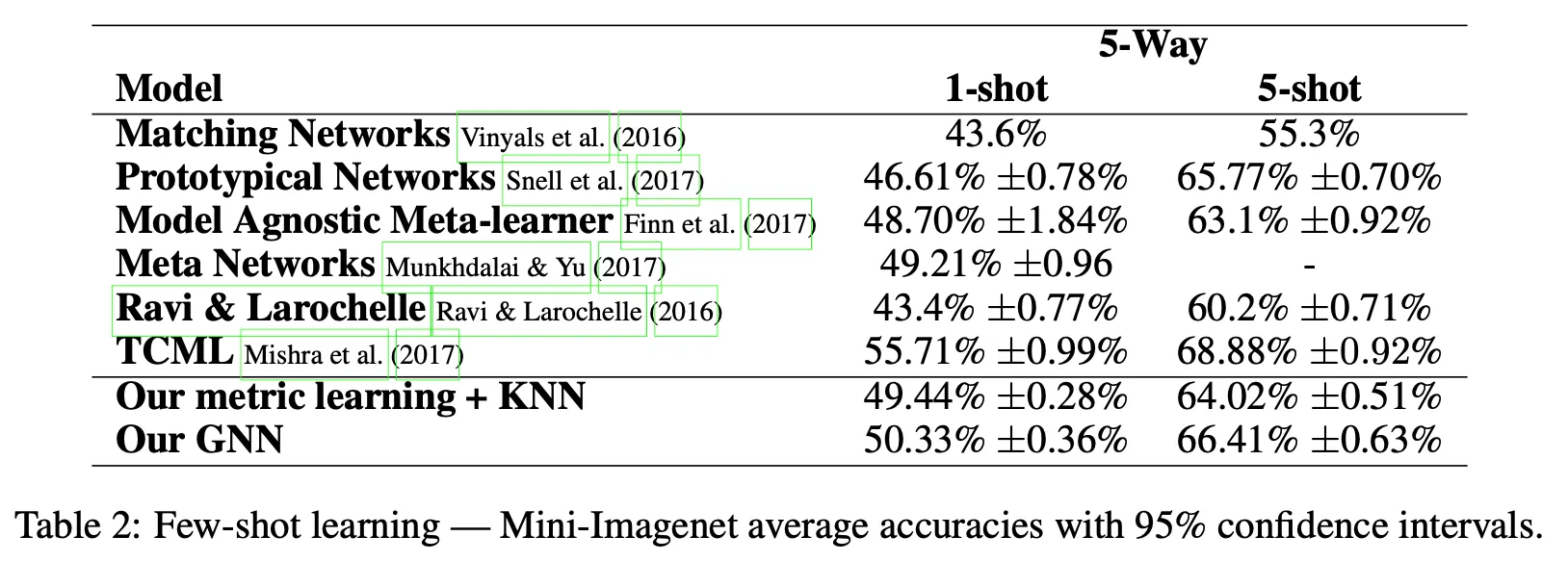
# of parameters: ,
Mini-ImageNet:
Originally introduced by Vinyals et al.(2016)
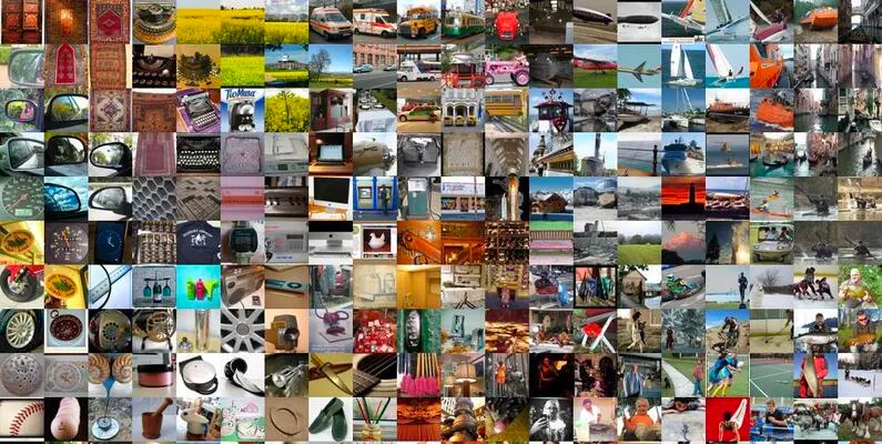
Mini-ImageNet
Divided into 64 training, 16 validation, 20 testing classes each containing 600 examples.
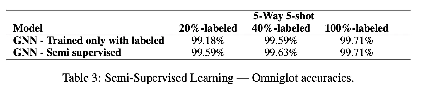
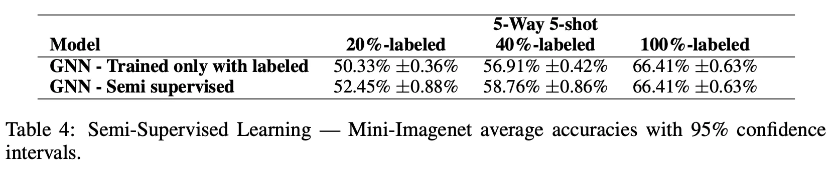
6.2. Semi-supervised learning
Omniglot
Mini-ImageNet
6.3. Active learning
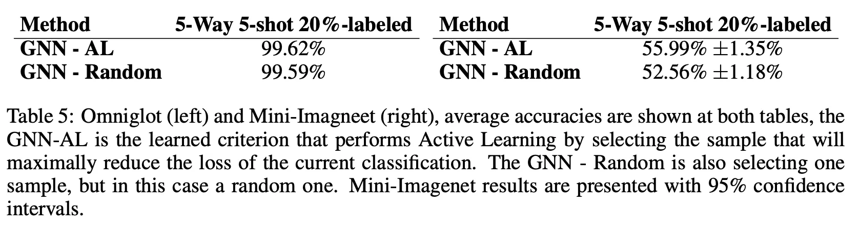
Random: Network chooses a random sample to be labeled, instead of one that maximally reduces the loss of the classification task