


1. Introduction
Many ML tasks are defined on sets of instances.
→ These tasks do not depend on the order of elements
→ We need permutation invariant models for these tasks
2. Major contribution
Set Transformer
•
Used self-attention to encode every element in a set.
→ Able to encode pairwise- or higher-order interactions.
•
Authors introduced an efficient attention scheme inspired by inducing point methods from sparse Gaussian process literature.
→ Reduced the computation to
•
Used self-attention to aggregate features
→ Beneficial when the problem requires multiple outputs that depend on each other
e.g.) meta-clustering
3. Background
Set-input problems?
Definition: A set of instances is given as an input and the corresponding target is a label for the entire set.
e.g.) 3D shape recognition, few shot image classification
Requirements for a model for set-input problems
•
Permutation invariance = order-independent
•
Input size invariance
c.f.) Ordinary MLP or RNNs violate these requirements.
Recent works
[Edwards & Storkey (2017)], [Zaheer et al. (2017)] proposed set pooling methods.
Framework
1.
Each element in a set is independently fed into a feed-forward neural network.
2.
The resulting embeddings are then aggregated using a pooling operation(mean, max, sum...)
→ this framework is proven to be a universal approximator for any set function.
→ However, it fails to learn complex mappings & interactions between elements in a set
e.g.) amortized clustering problem
Google search
Amortized clustering: Reusing the previous inference (clustering) results to accelerate the inference (clustering) of new dataset.
Pooling architecture for sets
Universal representation of permutation invariant functions
The model remains permutation-invariant even if the "encoder" is a stack of permutation-equivariant(order-dependent) layers
e.g.) permutation-equivariant layer - order matters!
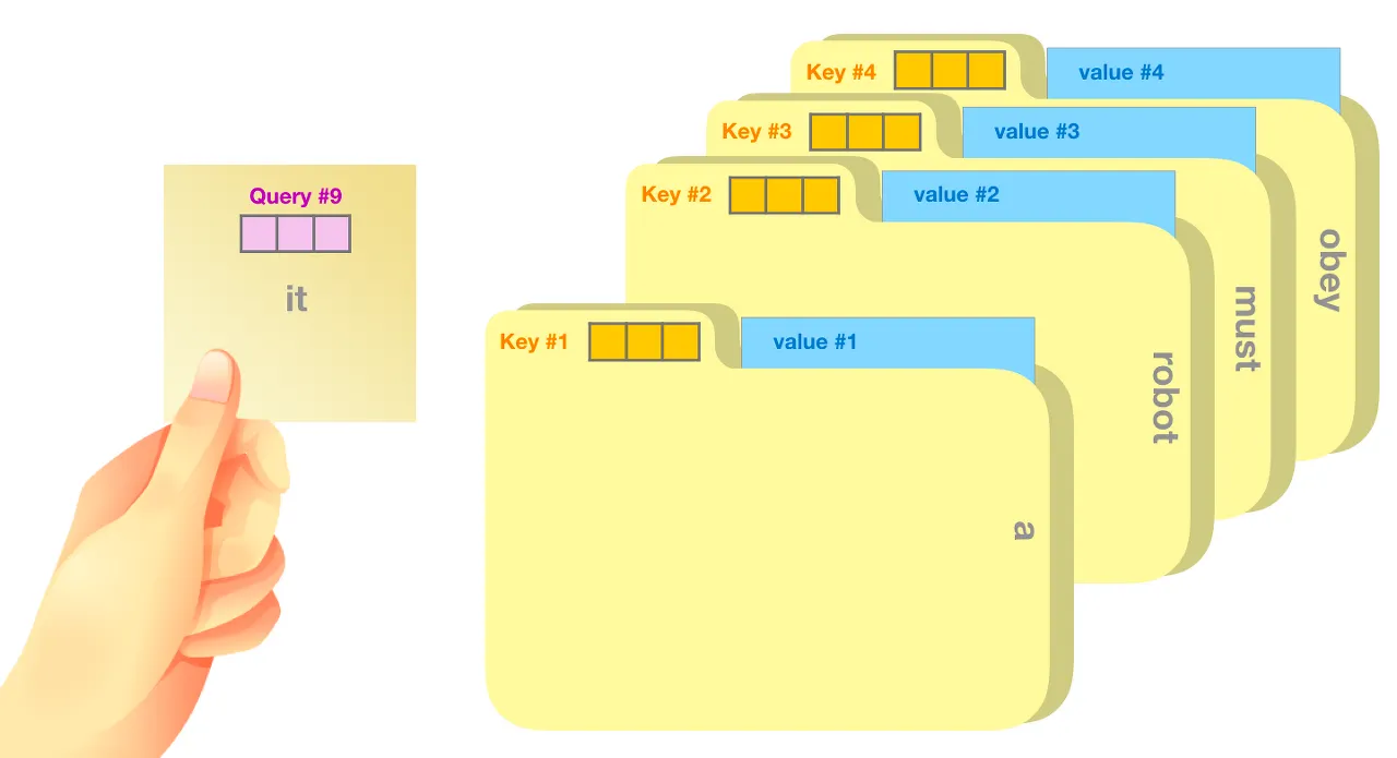
Attention
A set with elements = query vectors of dimension each →
An attention function maps queries to outputs using key-value pairs
→ measures how similar each pair of query and key vectors is.
usually,
from huidea_tistory
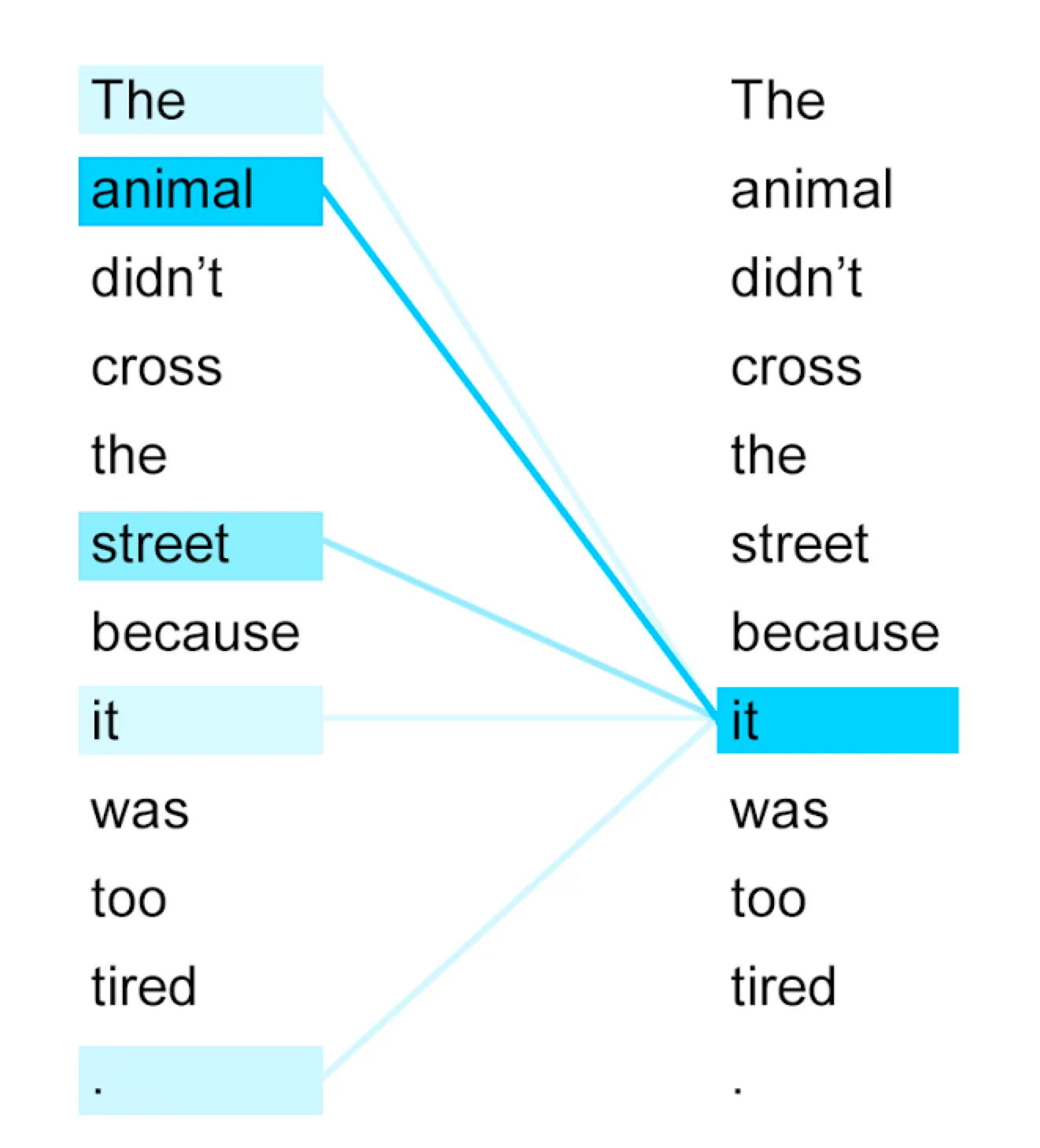
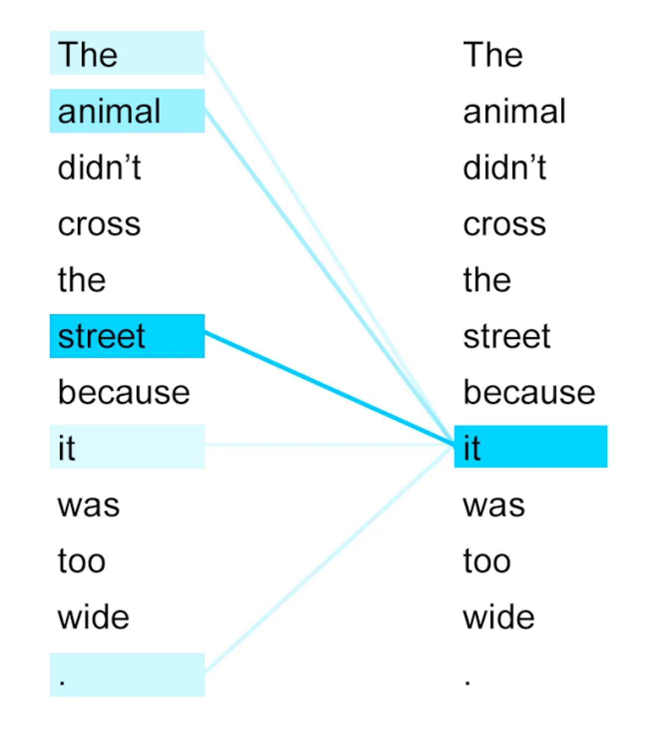
Self attention
From Google AI Blog
From Google AI Blog
•
Attention:
•
Self-attention:
→ Can approximate interactions between input data
Multi-head self-attention
Instead of computing a single attention function, this method first projects onto different -dimensional vectors
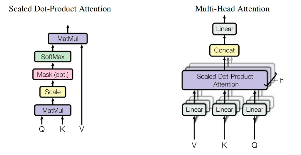
From Attention is all you need
4. Deep-dive
4.1. Permutation equivariant (induced) set attention blocks
4.1.1. Taxonomies
→ Matrix
→ processes each instance independently and identically

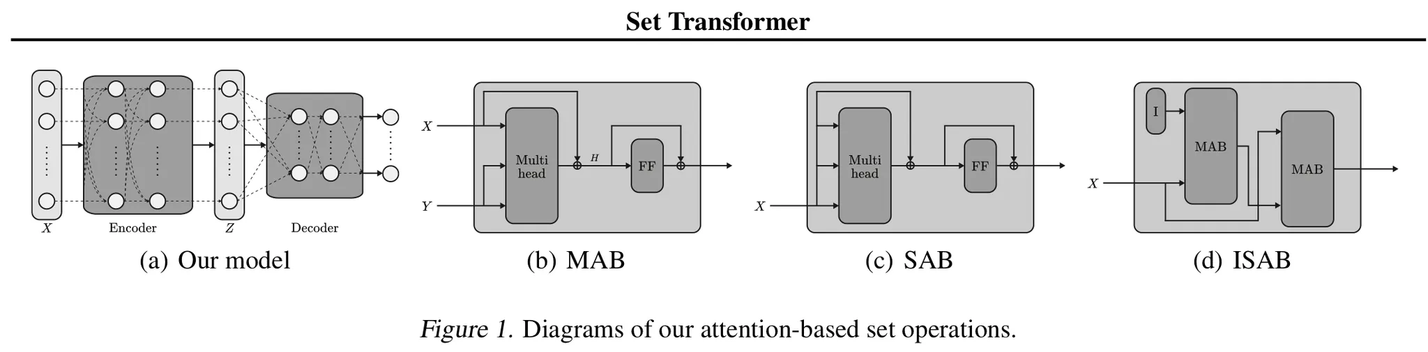
4.1.2. MAB
c.f.) is an encoder block of the Transformer without positional encoding and dropout
4.1.3. SAB
A special form of MAB
→ takes a set and performs self-attention.
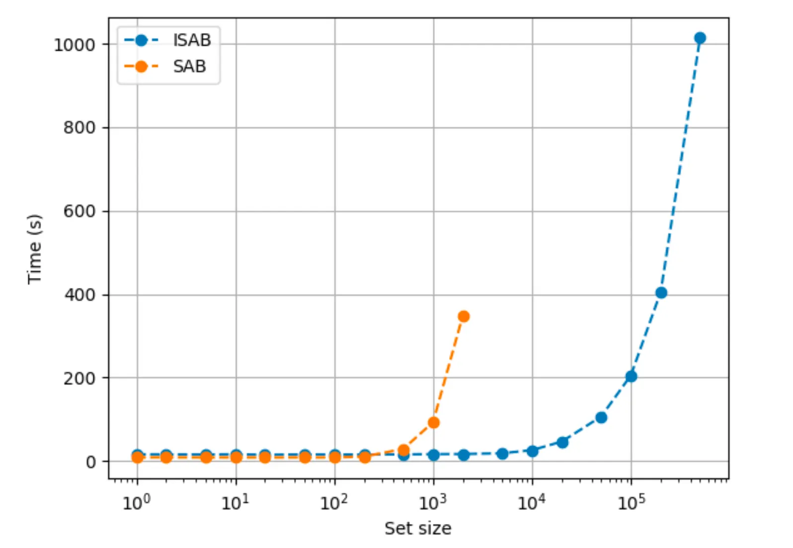
But, a potential problem of using SABs is the quadratic time complexity
→ Authors introduce the ISAB(Induced Set Attention Block)
4.1.4. ISAB
Additionally define -dimensional vectors ← trainable parameters
1.
Transform into by attending to the input set.
2.
: the set of transformed inducing points, which contains information about , is again attended to by to finally produce a set of elements.
→ Similar to low-rank projection or autoencoder, but the goal of ISAB is to obtain good features for the final task.
e.g.) In amortized clustering, the inducing points could be the representation of each cluster.
Time complexity of ISAB is → Linear!
4.2. Pooling by Multi-head attention
Common aggregation scheme: dimension-wise average or maximum
Instead, authors propose applying multi-head attention on a learnable set of seed vectors . is the set of features constructed from an encoder.
with seed vectors
Output of is a set of items.
In most cases,
But for tasks such as amortized clustering which requires correlated outputs, we need to use seed vectors
To further model the interactions among the outputs, authors apply SAB
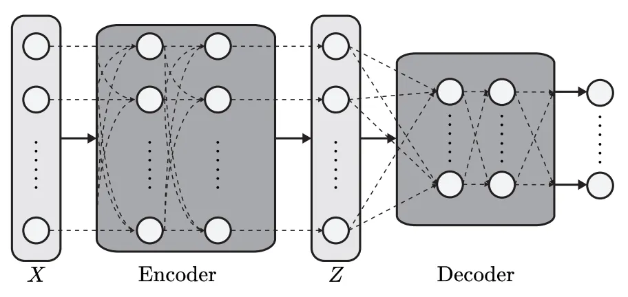
4.3. Overall Architecture
Need to stack multiple SABs to encode higher order interactions.
Time complexity for stacks of SABs and ISABs are and
Decoder aggregates into a single or a set of vectors which is fed into a feed-forward network to get final outputs.
4.4. Analysis
The encoder of the set transformer is permutation equivariant.
But the set transformer is permutation invariant.
5. Experiments
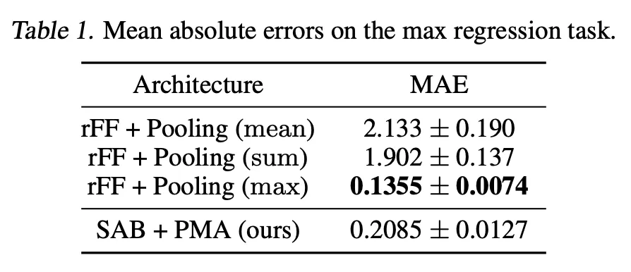
5.1. Toy problem: Maximum value regression
Motivation: Can the model learn to find and attend to the maximum element?
The model with max-pooling can predict the output perfectly by learning its encoder to be an identity function.
Set transformer achieves comparable performance to the max-pooling model.
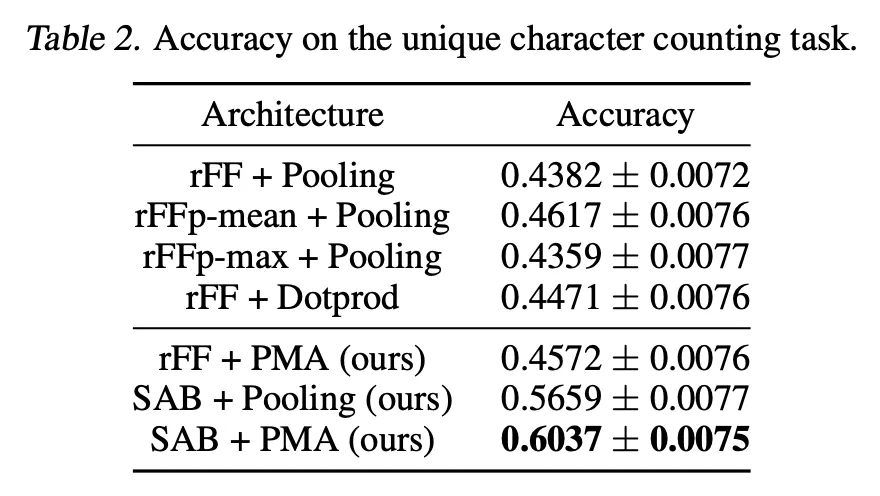
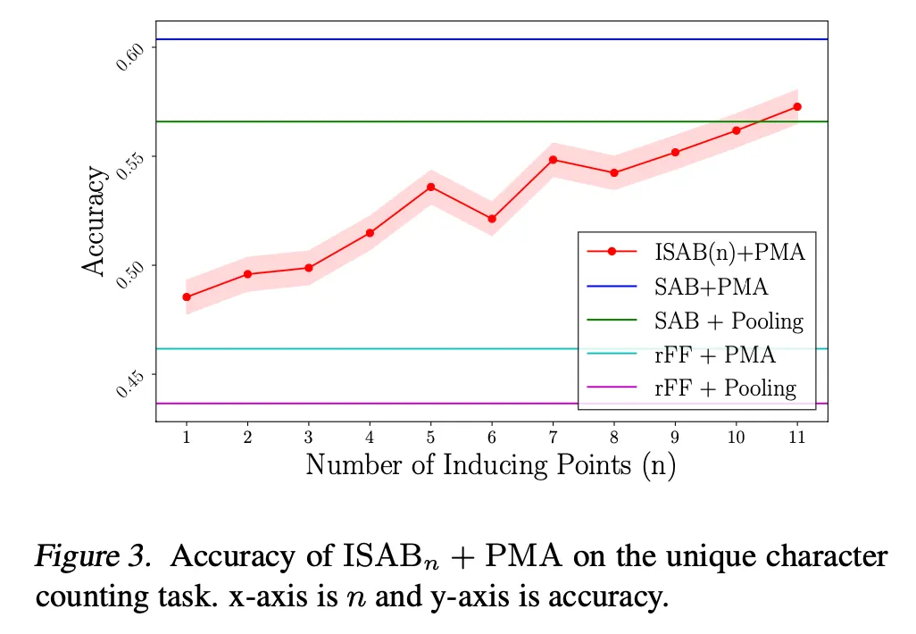
5.2. Counting unique characters
Motivation: Can the model learn the interactions between objects in a set?
Dataset: Omniglot
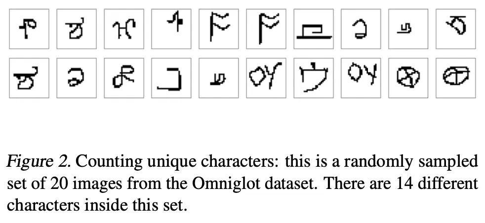
Goal: Predict the number of different characters inside the set
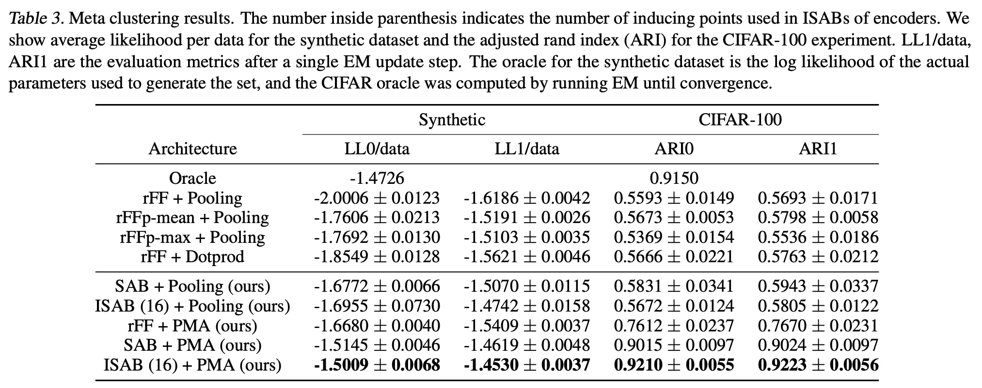
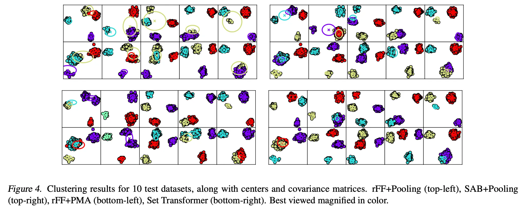
5.3. Amortized clustering with mixture of Gaussians
The log-likelihood of a dataset
Typical approach is to run an EM algorithm until convergence.
Dataset:
•
Synthetic 2D mixtures of Gaussians
•
Vectors from pretrained VGG network trained on CIFAR-100
Goal: Learn a generic meta-algorithm that directly maps the input set to
6. Conclusion
Why I chose this article
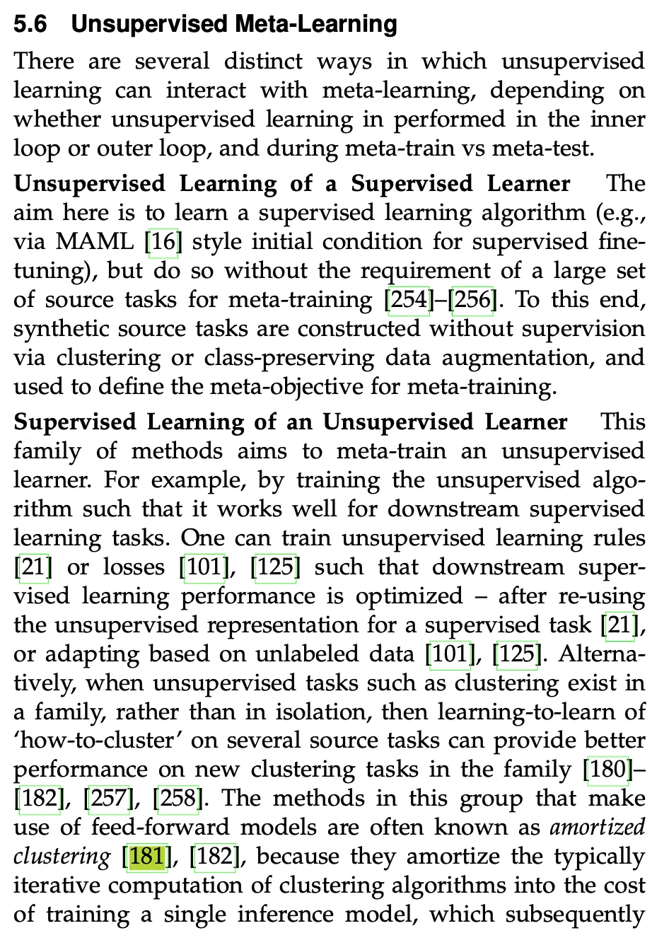
From Meta Learning in Neural Networks: A Survey
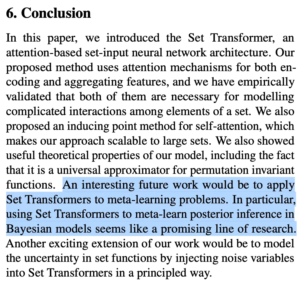
From Set Transformer