Protein-Protein Docking: Past, Present, and Future

Protein-Protein Docking: Past, Present, and Future [Paper]

Summary

1. Introduction

2. Protein Representation Schemes

3. Protein-Protein Docking: A General Pipeline

3.1. Pose generation (= sampling)

3.2. Scoring

4. Algorithmic Approaches in Protein-Protein Docking

4.1. Computational geometric algorithms

4.2. Population based metaheuristic algorithms

4.3. Monte Carlo algorithms

4.4. Graph based algorithms

4.5. Machine learning based algorithms

4.6. Deep learning techniques

5. Implementation Aspects: Parallel Computing in Docking

6. Critical Assessment of Prediction of Interactions (CAPRI)

7. Benchmask set and Evaluation Criteria

8. Discussion

8.1. Challenges and future in deep learning techniques

9. Conclusion

Summary

•

제목 그대로, protein-protein docking의 과거, 현재 (2021년 기준), 미래에 대해 다룹니다.

•

실제 연구를 수행할 때 눈여겨 볼 만한 부분은 회색과 갈색으로 표시해두었습니다.

1. Introduction

그동안 단백질 구조 결정에 사용한 기법들

	X-ray	NMR
장점	비용이 저렴 높은 해상도	Interaction dynamics 관찰 가능
단점	결정 구조를 만들어야 함 Conformation change를 modeling 하기 어려움	거리 기반이라 큰 단백질 관찰 어려움 (50 kDa 보다 큰 것은 거의 불가능)

Cryo-EM의 등장으로, 더 큰 단백질에 대해 찍을 수 있게 됨.

여전히 알려진 단백질 개수 >> 구조를 알고 있는 단백질 개수

단백질 구조 예측은 template-based / template-free로 구분 가능

단백질 Docking은 여러 interaction pattern 관찰 가능.

Rigid-body의 가정: 각 단백질이 internal geometry 유지한다.

→ 그렇지만 사실이 아님. side chain atom의 position 이 바뀔 수 있음.

MD, MC, NMA 방법들이 이런 conformational change 반영하는데 사용되고 있음.

단백질의 아미노산이 결합하는 양상을 파악할 수 있는 방법의 예시: Ramachandran plot

대부분 특정 angle range 안에서 결합한다.

이 plot만 가지고 구조의 품질을 판단하기는 어렵다.

2. Protein Representation Schemes

사람 몸에서 가장 큰 단백질: titin (27,000 ~ 33,000개의 아미노산)

얼마나 자세히 modeling 할 것인지 (full atom vs 일부)가 모델링에 드는 시간과 정확도에 크게 기여한다.

Coarse grained representation의 예시

•

Zacharias et al.: 각 residue 나타낼 때 하나는 CαC\alphaCα, 1~2개 pseudo atom은 side chain

•

Kolinski et al.: Cα−CβC_\alpha - C_\betaCα​−Cβ​ Side group (CABS) model 제안. 4개의 atom이 CαC_\alphaCα​, CβC_\betaCβ​, 2개의 pseudo atom이 두 CαC_\alphaCα​의 center & side chain의 center of mass 나타냄.

•

Khalili et al.: UNited RESidue model 제안. 두 개의 atom만으로 표현: CαC_\alphaCα​, side chain의 center of mass

•

AWSEM: 세 개의 atom: CαC_\alphaCα​, CβC_\betaCβ​, OOO

3. Protein-Protein Docking: A General Pipeline

Preprocessing - Sampling (pose generation) - Scoring - Refinement

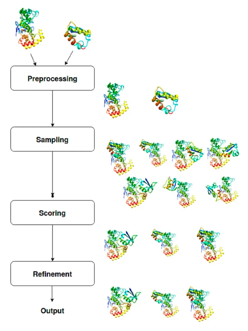
Pre-processing은 주로 MODELLER에 의해 수행됨.

input protein의 구조 다지기, missing atom/residue 처리

3.1. Pose generation (= sampling)

주로 단백질끼리의 translation, rotation을 고려한다.

크게 두 가지 방법으로 진행: Exhastive / Stochastic

•

Exhastive method:

매우 큰 seach space → 시간 오래 걸림. 여러 constraint (shape complementarity, electrostatic complementarity 등)를 줘서 space를 줄여줘야 함.

•

Stochastic method:

Random성에 의존. Metaheuristic algorithm과 함께 사용하기 좋음..?

3.2. Scoring

크게 다섯 가지 방법: Force-field / knowledge / empirical / consensus / machine learning

Force-field: 비공유결합 관련(van der Waals 나 electrostatic potential) + 공유결합 관련(bond angle, bond length, dihedral angle, ..) 모두 사용하지만, 단백질-단백질 rigid docking에서는 비공유결합관련 factor들만 활용. 일부 flexible docking 시에는 공유결합 관련 factor 활용하기도 함.

Knowledge-based: 이미 알려진 데이터 바탕으로 통계적인 방법 활용

4. Algorithmic Approaches in Protein-Protein Docking

Computational complexity가 높기 때문에, 여러 알고리즘들이 개발되어 사용되고 있다.

각 subsection 마다 선행연구들이 중구난방으로 적혀있는데 pose generation (sampling), scoring 등 다양한 곳에 사용되는 알고리즘을 정리한 것으로 볼 수 있다.

4.1. Computational geometric algorithms

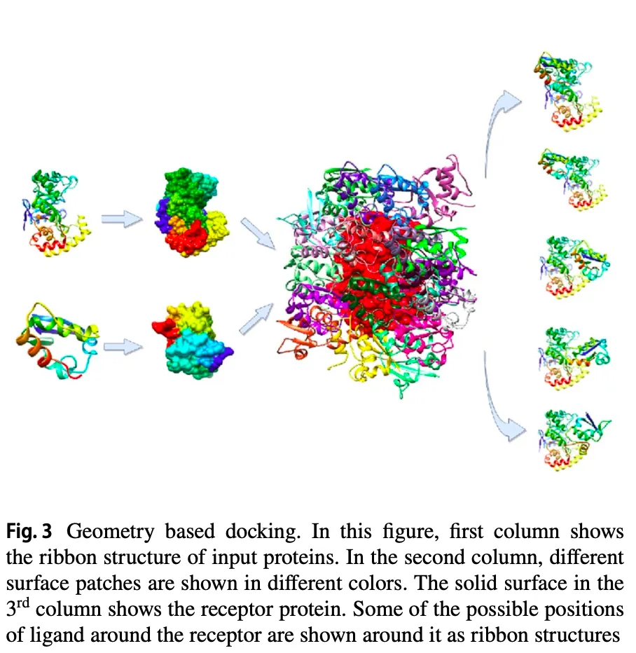
Interface region의 shape complementarity (상보성)을 이용.

그러나 protein-ligand의 경우 일종의 lock-key 전략이 통하지만, protein-protein 의 경우 이 constraint가 심하지 않음.

Rigid-body target에 대해서는 상보성이 높게 모델링하지만, antigen-antibody target에 대해서는 좀 더 relaxed 전략을 적용함.

단백질의 특정 부분들을 convex, concave, flat으로 구분하고 pose generation에 활용하기도 한다.

Shape descriptor가 충족해야 할 조건

•

Translation and Rotation invariance

•

Statistical independence

•

Reliable and fast

4.2. Population based metaheuristic algorithms

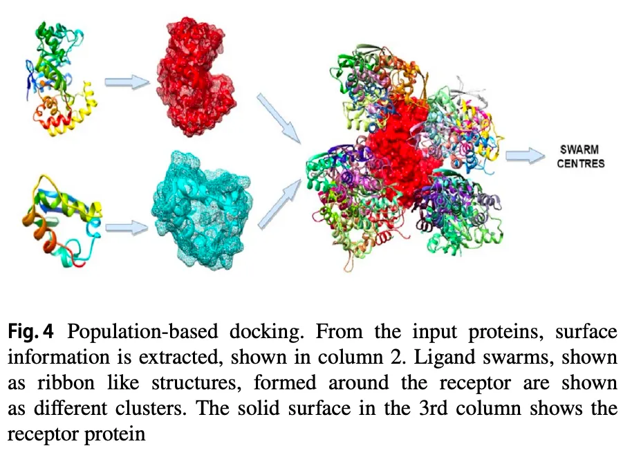
단백질 간의 중요한 interaction:

•

van der Waals force

•

electrostatic force

•

desolvation potential

→ 이런 interaction 잘 고려해서 minimum energy 가지는 pose 찾아야 함.

•

Evolutionary algorithms: balance exploration & exploitation

◦

Gardiner et al.: Genetic algorithm 기반의 protein-protein docking

◦

Sunny et al.: Flower Pollination Algorithm 기반의 FPDock 제안

◦

SwarmDock: Particle Swarm Optimization (PSO)와 normal mode analysis 활용

◦

JabberDock: MD simulation + PSO sampling

◦

Jimenez Garcia et al.: LightDock. Glowworm Swarm Optimization (GSO) 활용. Quaternion 으로 rotation 정의

4.3. Monte Carlo algorithms

Historical data 기반으로 probability value 예측

Randomness에 의존하여 non-deterministic solution 제공.

4.4. Graph based algorithms

단백질 구조를 graph 형태로 표현해서 모델링.

Sampling 관련 연구들

•

Grindley et al.: maximum common subgraph (MCS) 기반으로 complementarity finding 제안.

•

Gardiner et al.: MCS의 idea를 활용해 shape과 hydrogen bonding complementarity 기반으로 binding region 찾는 것을 제안.

•

Axenopoulous et al.: ligand surface와 receptor surface의 negative 고려..?

•

SP-Dock: shape complementarity 기반의 docking tool

Scoring 관련 연구들

•

TreeDock: multi-dimensional binary search tree로 protein의 energy landscape 탐색

•

Borgwardt et al.: GraphRank를 활용한 subgraph similarity search로 protein function 예측

•

Geng et al.: GraphRank로 best docking model 찾는데 사용. iScore 라는 tool로, SVM 써서 positive/negative 구분.

4.5. Machine learning based algorithms

초반부는 machine learning에 대한 개요 (supervised/unsupervised learning, RL, …)를 다룸.

4.6. Deep learning techniques

초반부는 deep learning에 대한 개요를 다룸.

CNN-based

•

Townshend et al.: SAS-Net. 단백질 atom의 spatial info 사용 → interfacial residue 예측

이 연구에서는 Database of Interacting Protein Structures (DIPS) 라는 dataset도 제공했음 → 이후 EquiDock이나 DiffDock-PP에서 사용됨.

•

Xie et al.: 서열 정보 + sequence profile + 물리화학적 성질 + 구조적인 정보 → residue의 interaction propensity 예측

•

Zhu et al.: ConvsPPIS. 서열 + 진화적 정보 + 구조 데이터 → feature graph 만듦 → CNN + ensemble predictor로 interface residue 예측

•

Hadarovich et al.: CNN으로 Homodimer의 구조 예측

•

DOcking decoy selection with Voxel-based deep neural nEtwork (DOVE): 3D CNN으로 PP docking. Dataset에서 redundant한 것들을 없애기 위해 TMscore 사용.

GNN and GCN

•

Fout et al.: GCN 기반의 모델로, 각 residue pair가 interacting 하는지 안 하는지 예측

•

Xie et al.: Residue binding propensity를 더해주는게 효과적.

•

Liu et al.: 구조 정보 + 서열 정보 + high order interaction data (adjacent residue pairs) 활용

•

Cao et al.: GCN 기반 scoring. Intra- & inter-molecular contact map을 input으로 받음 → intra & inter-protein energy value 계산. 모델은 계산된 Gibbs energy와 complex의 실제 energy 차이를 출이도록 학습. Output score는 affinity prediction에 사용.

•

Wang et al.: GNN 기반 scoring. Graph에 interfacial information embed.

Generative models

•

Degiacomi: 단백질 구조 생성에 autoencoder 활용

•

Ramaswamy et al.: Autoencoder에 1D convolution 적용 → conformation space generation을 개선. Physics term들이 성능 항상에 도움을 줌.

•

Nguyen et al.: GAN 활용.

Others

•

Tensor field networks: translation, rotation invariance 줄 수 있음.

◦

Eismann et al.: PAUL이라는 scoring 방법. Atom level feature로 3D 좌표, atom 이름, receptor인지 아닌지 만 사용. Local neighborhood에서 physical force 반영. Ligand RMSD prediction task 수행.

◦

Gainza et al.: Surface를 fragment로 나눠서 biophysical & chemical/structural property 할당 → interaction 예측. MaSIF-site (두 단백질 간 interaction site 예측), MaSIF-ligand (ligand의 binding pocket 예측), MaSIF-search (가장 그럴듯한 interaction filter out).

5. Implementation Aspects: Parallel Computing in Docking

Hardware의 발달(특히 GPU)로 병렬 컴퓨팅이 많이 발전했다.

병렬 컴퓨팅을 잘 활용한 연구의 예시

•

MegaDock 4.0: Katchalski-Katzir에 의해 제안된 방법을 활용해 generated pose의 score 예측. 모든 process (voxelization, ligand tranformation, score calculation, final prediction)에 GPU를 사용함.

•

Cell-Dock

•

Sukwani et al.: PIPER (FFT 기반 알고리즘)을 가속화.

6. Critical Assessment of Prediction of Interactions (CAPRI)

CAPRI는 EMBL-EBI가 주최한 PP-docking 대회. Input protein들의 좌표를 주고, 10개의 complex 구조 예측하도록 함.

2014년부터는 CASP와 공동 주최 → CASP-CAPRI 로 열리기 시작함.

cf) CASP은 2년마다 열리는 단백질 구조 예측 대회.

대부분의 target들은 homo-oligomer.

대부분의 참가자들은 초반에 template-free 방법을 사용했다가, clustering technique이 소개됨에 따라 비슷한 구조들을 참고하여 성능 개선하였음.

이후 추가적인 task도 만들어서 함께 수행: interfacial water molecule 위치 예측, binding affinity 예측.

•

Lensink et al.: 2019년에 열린 CASP13-CAPRI에 소개된 method들을 정리함.

◦

Cluspro: HHPred 사용해서 적절한 template 얻음. Template 얻기 어려운 경우엔 free docking 활용 (FFT 기반의 PIPER algorithm). 생성된 구조는 van der Waals, electrostatic, desolvation potential로 scoring. 최종적으로 구조의 중심을 찾고, CHARMM potential을 활용한 van der Waals minimization을 통해 atomic clash 최소화.

◦

MDockPP: FFT 기반 구조 생성 → optimization → scoring (with ITScorePP)

◦

GalaxyPPDock: GalaxyHomomer를 기반으로 하여 HHSearch로 template을 알아냄. FFT 기반의 ab initio docking 수행, GalaxyRefineComplex를 활용해 구조 refinement.

◦

PSO 기반 구조 예측 방법들은 HHBlits 활용해 homologous sequence 알아내고 각각의 구조를 PSO^2로 생성. 이후 SwarmDock algorithm 활용해 optimal binding location 찾고 SVM으로 ranking.

◦

HADDOCK: 세 가지 (ab initio, template-based, information-driven) 방법 사용했으나, ab initio 는 제대로 작동하지 않았음.

◦

LZerD: 적절한 template이 있는 경우에만 사용가능.

7. Benchmask set and Evaluation Criteria

Benchmark set

자주 쓰는 PP docking benchmark: DOCKGROUND, PPI4Dock

•

Chen et al. (2003): PP docking benchmark 제안. 여러 난이도 (rigid-body, medium, difficult). 계속 업데이트되고 있으며, 가장 최근 version 5.5는 162개 rigid body, 60개 medium difficulty, 35 difficult target 포함. 실험적으로 만들어진 구조들이고, 모두 bound & unbound 얻을 수 있음.

•

DOCKGROUND (2006): 실험적으로 얻은 구조 뿐만 아니라 계산으로 얻은 bound & unbound 구조도 포함됨. X-ray bound, X-ray unbound, simulated unbound, model-model complexes, X-ray docking decoy, docking template 이 제공됨. Computational unbound 구조는 Langevin dynamics simulation에 의해 만들어짐. Decoy 구조는 GRAMM-X로 만들어짐.

•

PPI4Dock: 비교적 큰 docking dataset. Homology modeling 으로 1417 target 보유. Original crystal 구조에 대해 template structure의 deviation에 따라 easy, very easy, hard, very hard, super hard로 분류.

•

DIPS (2019): Townshend et al. 에서 제안한 PP docking benchmark dataset. 42,826개의 binary protein complex 존재.

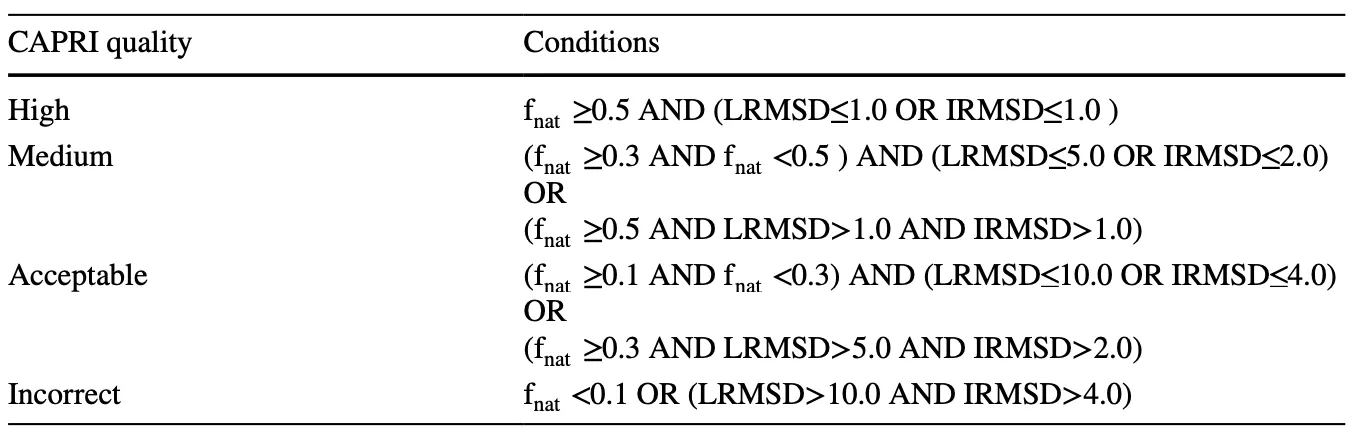
Evaluation criteria

CAPRI evaluation criteria (LRMSD, IRMSD,

\text{f}_{\text{nat}}

)를 자주 사용.

•

LRMSD: root mean square deviation of ligand backbone atoms

•

IRMSD: root mean square deviation of interface atoms

•

fnat\text{f}_{\text{nat}}fnat​: fraction of native residues (native 구조 대비 predicted 구조에서 interface residue가 몇 개나 되는지)

•

최종적으로 아래의 기준으로 high / medium / acceptable / incorrect 로 분류

DockQ score: 위 기준표가 robust하지 않다고 해서 나온 metric. 0과 1사이의 값.

DockQ = (\text{f}_{\text{nat}} + LRMSD_{\text{scaled}} + IRMSD_{\text{scaled}})/3

where

RMSD_{\text{scaled}} = \frac{1}{1 + \big(\frac{RMSD}{d_i}\big)^2}

d_i

는 LRMSD는 8.5Å, IRMSD는 1.5Å

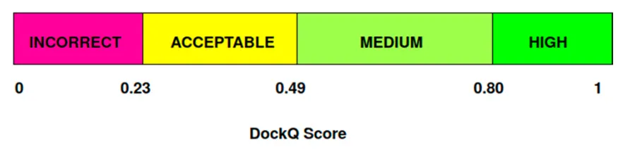
CAPRI에서도 DockQ score를 사용한다.

8. Discussion

•

Data quality

Data input으로는 대부분 high-quality X-ray 구조를 선호하지만, 그 수가 적다.

따라서 low-quality 구조도 사용해야 하는데 이때 small angle X-ray scattering (SAXS)나 homology modeling으로 얻은 구조가 유용하게 쓰일 수 있다.

•

Amount of information

◦

Docking algorithm을 쓸 때는 적절한 성능을 내기에 필요한 만큼의 정보만 사용하는 것이 좋다.

◦

HADDOCK-CG에 Martini force-field 사용할 경우 성능이 좋았다.

◦

Coarse-grained feature를 사용해서 energy landscape을 부드럽게 가져가고, 실행 시간도 빨라진다. Conformation의 작은 변화에도 덜 민감하다.

•

Computation cost

◦

주요 bottleneck은 score 계산과 refinement 단계이다. 이 부분을 줄이는게 중요하다.

◦

Protein-Protein interaction이 각 단백질의 core 부분에는 영향 X

→ 많은 방법들이 pairwise energy 계산 시 특정 depth에서만 계산해서 쓴다.

•

Water molecule

◦

Hydrogen-protein bond에 물 분자가 중요하게 관여한다. 이 물 분자들을 highly coordinated water molecule 이라고 부른다.

◦

이들의 contribution을 scoring function에 반영하는게 conformation space의 sampling을 개선한다.

◦

그리고 단백질끼리 가까이 다가갈 때, 그 닿는 부분의 물 분자들은 흩어질 것이므로, binding site를 알아내는데 주요하게 작용할 수 있다.

•

Evolutionary algorithm & SVM

◦

이 둘을 적용할 수 있는 부분에 잘 적용하는 것이 성능 향상에 도움이 된다.

•

Flexibility

◦

좋은 docking tool이 되려면 side chain과 backbone flexibility도 잘 반영할 수 있어야 한다.

◦

그러나 flexibility를 부여하는 것이 항상 좋은 구조 예측을 불러오는 것은 아니다. 특정 단백질은 rigid한 구조를 선호하기도 하기 때문이다.

◦

최근 modeling의 trend는 여러 타입의 데이터를 활용하는 것이다. X-ray, NMR, electron microscopy, footprinting, chemical crosslinking, FRET spectroscopy, SAXS, proteomics 등.

•

Template

◦

대부분의 경우에 적절한 template을 얻을 수 있다면, 그것을 활용하는 것이 좋다.

8.1. Challenges and future in deep learning techniques

ML → DL로의 transition은 GPU의 발달과 관련이 깊었다.

ML model들은 사람이 handcrafted feature를 잘 선별해줘야 했지만, DL model들은 raw data에서 직접 feature를 뽑아낸다.

DL의 major hurdles

•

Data representation

◦

atom간의 positional information & interaction

◦

단백질의 3D 좌표 상의 positional detail, sparsity

◦

Graph로 표현 시 location 정보를 어떻게 넣어줄지 (atom/residue간 direction 등을 node feature로)

◦

Sequence를 다룰 경우 BERT나 Transformer 활용하면 좋음.

•

Overfitting & underfitting issues

◦

Data distribution을 손봐줘야 한다.

•

Hyperparameter tuning

•

Computational limitations (hardware)

GAN이나 tensor field network를 잘 활용해보자.

Sequence로부터 protein complex structure prediction 하는 방향도 생각해보자. AlphaFold 처럼 self-attention을 잘 활용.

9. Conclusion

Conventional technique은 상대적으로 data가 적은 상황에서 잘 작동. 주로 physicochemical & geometric property 분석해서 near-native 구조를 맞추도록 함.

점점 더 많은 protein complex의 구조가 밝혀짐에 따라 template을 활용하는 방법들이 발달.

최근에는 deep learning을 활용하는 연구들이 많아졌고, 이들을 잘 학습하기 위해서는 더 많은 양의 데이터가 있어야 할 것.