DiffDock-PP: Rigid Protein-Protein Docking with Diffusion Models

DiffDock-PP: Rigid Protein-Protein Docking with Diffusion Models [Paper] [Code]

Summary

1. Introduction

2. Background and Related Work

3. Method

4. Experimental Setup

5. Results

6. Conclusion

7. Major Takeaways

Summary

이 논문의 Contribution은 무엇일까?

•

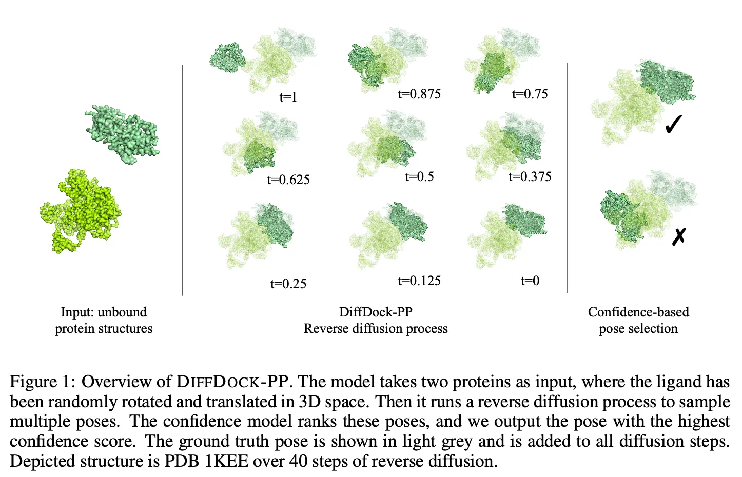
DiffDock (protein-ligand docking. ICLR 2023)을 기반으로 하여 protein-protein docking (PP docking) 문제를 접근함.

•

Score model:

Translation과 rotation에 각각 적합한 diffusion process를 활용한 generative problem으로 docking pose generation을 수행함.

•

Confidence model:

생성된 docking pose의 L-RMSD가 특정 threshold 미만일지 아닐지 binary classification 수행함.

•

일부 PP docking에서 SOTA 성능 달성

1. Introduction

생체 내에서 단백질의 기능과 역할은 단백질의 구조와 밀접한 연관이 있다.

각 단백질은 다른 단백질, 핵산, 저분자화합물 등과 결합하면서 여러 기능을 수행한다.

따라서 protein-protein docking (PP docking)을 잘 수행하는 것이 중요하다.

DiffDock-PP는 PP docking 시에 rigid body를 가정하고 진행한다.

Rigid body 란?

•

각 단백질의 internal bond angle과 torsional angle 등이 움직이지 않고 고정되어 있다는 것을 의미한다.

•

Unbound state과 bound state을 비교해보면 각 단백질의 구조가 고정되어 있지는 않지만, 문제를 쉽게 풀기 위해 가정을 하고 진행하는 경우가 많다. 2014년 리뷰 논문 (Vakser et al.)에 따르면, 대부분의 경우에 unbound/bound 구조가 큰 차이는 없다고 한다 (DOCKGROUND 데이터셋 기준 RMSD <2Å 미만인 것이 70% 이상). 물론 side chain 등까지 고려했을 때는 그 차이가 커질 수 있다고 한다.

•

어떻게 하면 이 가정을 하지 않고도 좋은 성능을 낼 수 있을지 고민해보자.

PP docking의 전통적인 방법들은 주로 two-step으로 접근했다.

Search algorithm: 

Potential pose 생성. Search space가 매우 넓어 오래 걸린다.

Scoring function: 

생성된 pose들 중 괜찮은 것들을 선택하기 위한 기준점이 될 점수를 계산한다.

최근에는 Deep learning 방법들이 제안되고 있다.

•

EquiDock (Ganea et al. 2021):

Regression 기반의 PP docking. 속도는 빠르지만 전통적인 방법들의 성능을 뛰어넘지는 못 했다.

DiffDock-PP는 diffusion 기반의 generation으로 접근하며, Database of Interacting Protein Structures (DIPS) 데이터셋에서 SOTA 성능을 달성했고, 전통적인 방법들 대비 5~60배 이상 빠른 속도를 보여준다.

2. Background and Related Work

Protein-Protein Docking

정의: 개별 unbound 구조들로부터 bound 구조를 예측하는 것.

DiffDock-PP는 rigid body docking을 수행한다. 이 가정은 꽤나 잘 작동한다고 한다.

일반적으로 성능 평가는 특정 threshold distance 이내에 들어오는 구조들의 개수, 또는 비율 (fraction) 로 평가한다.

(Traditional) Search-based Docking Methods

이전엔 어떤 방법들이 있었나?

PP docking의 전통적인 방법들은 complex의 물리적인 특성들을 이용했다.

그럴듯한 complex 구조들을 여러 개 생성

Optimization algorithm을 활용해 구조 최적화

Scoring function으로 점수를 매겨 높은 점수의 complex 선택

Template-based modeling 방법들도 함께 사용되었다.

이 방법들은 오래 걸려서 large-scale screening에 적용되기에는 한계가 있다.

(Recent) Deep Learning-based Docking Methods

최근엔 어떤 방법들이 소개되었나?

크게 single-step / multi-step method로 구분된다.

•

Single-step method: 한 번에 complex 구조를 예측한다.

◦

EquiDock (Ganea et al. 2021): SE(3)-equivariant graph matching network를 활용해 regression으로 접근했다.

◦

dMaSIF-dock (Sverrison et al. 2022): Energy 기반 model에 physical prior 도입

•

Multi-step method: 최종 구조를 얻기 위해 iterative refinement를 수행한다.

◦

AlphaFold-multimer (Evans et al. 2021): Primary sequence와 multiple sequence alignment (MSA) 기반으로 complex 를 접는다.

◦

DockGPT (McPartlon & Xu, 2023): Generative protein transformer를 활용해 flexible & site-specific protein docking 수행했다.

DiffDock-PP는 diffusion을 사용했기 때문에 multi-step method의 일종이다.

Diffusion Generative Models (DGMs)

DGM이 무엇인가?

Diffusion process의 main idea: data distribution을 tractable prior로 바꿔서, score function을 학습하는 것.

Score function:

\nabla_\mathbf{x} \log p_t(\mathbf{x})

즉, log probability density function의 gradient이다.

이 score를 활용하면 probability distribution function에서 sample해서 data를 만들 수 있다.

이 diffusion process는 여러 computational biology task (conformer generation, molecule generation, protein design 등)에 사용되었다.

3. Method

Benefits of generative modeling for rigid protein docking

PP docking에 왜 generative model을 사용할까?

PP docking의 최종 성능 평가는 특정 threshold 미만에 존재하는 개수로 평가한다. 예를 들어, L-RMSD (ligand-RMSD) < 5Å 인지 또는 I-RMSD (interface RMSD) < 2Å 인지 등.

Original DiffDock 논문에서 다뤘듯이, 이 threshold 기반의 objective를 regression (MSE-type loss)에 접목하면 몇 가지 문제점이 있다.

Threshold-based objective는 미분이 불가능하다.

Regression은 multi-modality를 반영할 수 없다.

MSE loss는 steric clash가 발생하기 쉽다. (EquiDock)

→ Multi-modal distribution에서 regression을 사용하면 weighted mean으로 보내버린다.

from DiffDock

반면, 잘 학습된 generative model (data distribution을 잘 학습한)은 여러 mode에 가까운 것을 생성해낼 수 있다.

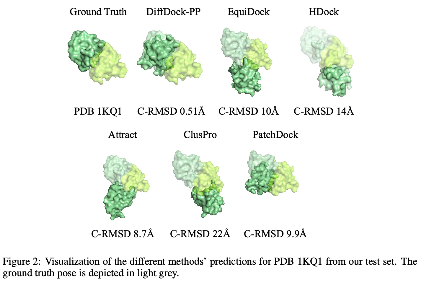
DiffDock-PP가 생성한 구조는 steric clash가 없다.

Method Overview

1. 단백질 구조를 어떻게 표현했을까? Full atom 또는 Coarse representation? 2. Docking에서 어떤 operation이 필요할까? 3. Docking을 수식으로 어떻게 표현할 수 있을까?

Protein structure representation

Protein을 residue level, 즉 각 residue의

C_\alpha

의 위치로 표현한다 (coarse representation)

\mathbf{X}_1 \in \mathbb{R}^{3n}

: ligand (

n

residues),

\mathbf{X}_2 \in \mathbb{R}^{3m}

: receptor (

m

residues)

본 논문에서는 두 protein 중 길이가 더 짧은 것 (residue 개수가 적은 것)을 ligand로 간주하고, receptor의 position은 고정했다.

즉, ground truth complex position을

\mathbf{X}^*_1 \in \mathbb{R}^{3n}

\mathbf{X}^*_2 \in \mathbb{R}^{3m}

라고 할 때,

\mathbf{X}_2 = \mathbf{X}^*_2

이다.

Operation

본 논문에서는 rigid body를 가정하므로, ligand의 rotation과 translation만 고려하면 된다.

	System	Degrees of freedom
Rotation	Euler angle (x, y, z 축 기준의 angle)	3
Translation	Euclidean vector (x, y, z vector)	3

수식

결국 하고자 하는 것은 확률 분포

p(\mathbf{X}_1 | \mathbf{X}_2)

를 학습하는 것이고, 이때

\mathbf{X}_1

(ligand)가 움직일 수 있는 manifold

\mathcal{M}

을 특정 operation이 수행될 수 있는 쪽으로만 제한한다.

Diffusion Process

1. 각 operation은 어떻게 수행되나? 2. 각 operation의 diffusion을 어떻게 정의할까?

Rotation & Translation

3D translation group:

\mathbb{T}(3)

, 3D rotation group:

SO(3)

→ 이 둘의 product space

\mathbb{P} = \mathbb{T}(3) \times SO(3)

우리가 정의하는 mapping

A: \mathbb{P} \times \mathbb{R}^{3n} \to \mathbb{R}^{3n}

A((r, R), x)_i = R(x_i - \bar{x}) + \bar{x} + r

이때

x_i

는

i

번째 residue의 위치이고,

\bar{x}

는 ligand의 center of mass이다.

Center of mass를 원점으로 보낸다. (그래야 rotation을 translation과 orthogonal하게 수행할 수 있는 것 같다.

Rotate

Center of mass를 원위치로 보낸다.

Translate

Diffusion on rotation & translation

DiffDock 논문에서 증명했듯이,

A(\cdot, \mathbf{X}_1): \mathbb{P} \to \mathcal{M}

은 bijection 이다. 즉, inverse가 항상 존재하는 1:1 mapping 이다. 따라서 각 operation의 manifold 상에서 diffusion을 수행하면 그것이 그대로 3차원 좌표계에 반영된다.

이는 각 operation이 flat Euclidean space가 아닌 Riemannian manifold에 존재하므로, 여기서 diffusion을 수행할 수 있다는 연구 (De Bortoli et al. 2022)에서 착안한다.

Diffusion은 denoising score matching network (Song & Ermon, 2019)을 사용하며, forward SDE는

d\mathbf{x} = \sqrt{d\sigma^2(t)/dt} \text{ } d\mathbf{w}

로 정의한다. 이때

\sigma^2

는 translation, rotation 각각 따로 정의하고,

d\mathbf{w}

는 Brownian motion을 의미한다.

Model Architecture

1. 어떤 네트워크 구조를 사용했을까? 2. 어떤 input feature를 사용해야 할까? 3. Convolution은 어떻게 수행할까? 4. 어떤 output을 내놓을까?

Network architecture

DiffDock과 비슷하게 SE(3)-equivariant convolutional network 사용.

Tensor field network (Thomas et al. 2018), Euclidean neural networks (Geiger et al. 2020) 참고.

이를 통해 protein-protein pair의 symmetry를 반영하고, rigidity assumption을 반영.

Input feature

각 protein은 heterogeneous geometric graph로 표현하고, 각 아미노산을 node로 표현.

•

Node feature:

◦

residue type

◦

position of CαC_\alphaCα​

◦

language model embedding (trained on ESM2)

•

Edges:

◦

Intra-edge: 같은 단백질 내에서 20개의 nearest neighbor끼리 연결

◦

Cross-edge: 다른 단백질끼리는 dynamic cutoff distance (40+3∗σtr)(40 + 3 * \sigma_{tr})(40+3∗σtr​)Å 를 적용해 edge 구축

▪

dynamic cutoff distance를 사용한 이유는 early diffusion step에서는 비교적 멀리 떨어져있더라도 서로 연결될 수 있도록하고, later diffusion step에서는 비교적 가까이 있는 것들만 연결해서 computational cost를 줄이기 위함! 

Intermediate layers

초기 feature와 diffusion time, edge length를 정한 뒤에 각 edge type (intra / cross) 마다 다른 convolution을 적용한다.

Output layers

Score model: tensor product convolution (center of mass에 대해)을 수행

→ 두 개의 3차원 SE(3)-equivariant vector (translational score, rotational score)

Confidence model: 마지막 layer에 mean-pool 이후 FC layer

→ 하나의 SE(3)-invariant confidence scalar value

Training and Inference

Diffusion model (score model)

Diffusion kernel과 score matching objective가 product space

\mathbb{P}

에서 정의되긴 했지만, Jing et al. 2022에서 제안한 extrinsic-to-intrinsic framework을 따라 training과 inference는 3D Euclidean space에서 수행한다.

DiffDock 때와 마찬가지로, 각 sample들은

(\mathbf{X}_1, \mathbf{X}_2)

로 구성되는데 conditional distribution으로 표현하면 각

p(\cdot|\mathbf{X}_2)

당 1개의 sample만 존재하는 상황이다.

따라서 training 시에는 서로 다른 conditional distribution에 대해 하나의 sample만 가지고 학습하게 되고, inference 시에는 low temperature sampling을 사용해 model이 mode들에 집중할 수 있도록 했다.

Confidence model

Confidence model은 L-RMSD 값이 5Å 미만인지 아닌지를 예측하는 binary classification으로 진행된다.

이를 학습하기 위한 training data는 학습된 diffusion model에서 생성한 여러 구조들에 대해 ground truth와 L-RMSD를 측정하고 5Å 미만인지 아닌지를 labeling 했다.

Combined inference

최종적으로 학습된 diffusion model로 여러 candidate pose를 sampling 하고, confidence model로 rank → 가장 높은 confidence score를 보이는 것을 선택했다.

4. Experimental Setup

Dataset:

Database of Interacting Protein Structures (DIPS) (Townshend et al. 2019) 사용. 이 dataset은 42,826개의 binary protein complex를 보유하고 있다.

본문에는 시간이 없어서 Docking Benchmark 5.5 (DB 5.5)에 대해서는 수행 못 했다고 되어있다.

Split:

EquiDock (Ganea et al. 2021)에서 사용한 protein-family 기반 split을 진행했다.

비교군 (baseline models):

Search-based baselines

•

ClusPro (FFT 기반) (Desta et al. 2020, Kozakov et al. 2017)

•

Attract (coarse-grained force-field 기반) (Schindler et al. 2017, de Vries et al. 2015)

•

PatchDock (shape complementary principle 기반) (Mashiach et al. 2010, Schneidman-Duhovny et al. 2005)

•

HDock (template 기반 모델링, ab initio free docking) (Yan et al. 2020, Huang & Zou 2014)

→ 이 네 개의 baseline model들의 train / test data는 control 할 수 없었다. 즉, 이 논문의 test set을 이 네 개의 baseline model들이 train 시에 봤을 수도 있다.

Deep learning baselines

•

AlphaFold-multimer (Evans et al. 2021)

•

EquiDock (Ganea et al. 2021)

성능 평가

•

EquiDock에서 제안한 evaluation scheme을 따랐다

•

모든 모델을 complex RMSD (C-RMSD)와 interface RMSD (I-RMSD)에 대해 평가했다.

◦

C-RMSD: ground truth와 predicted complex structure를 Kabsch algorithm으로 겹쳐서 CαC_\alphaCα​ 좌표끼리 RMSD 계산

◦

I-RMSD: 두 complex의 interface residue (< 8Å 미만의 거리에 있는 것들)를 align해서 interface CαC_\alphaCα​ 좌표끼리 RMSD 계산

5. Results

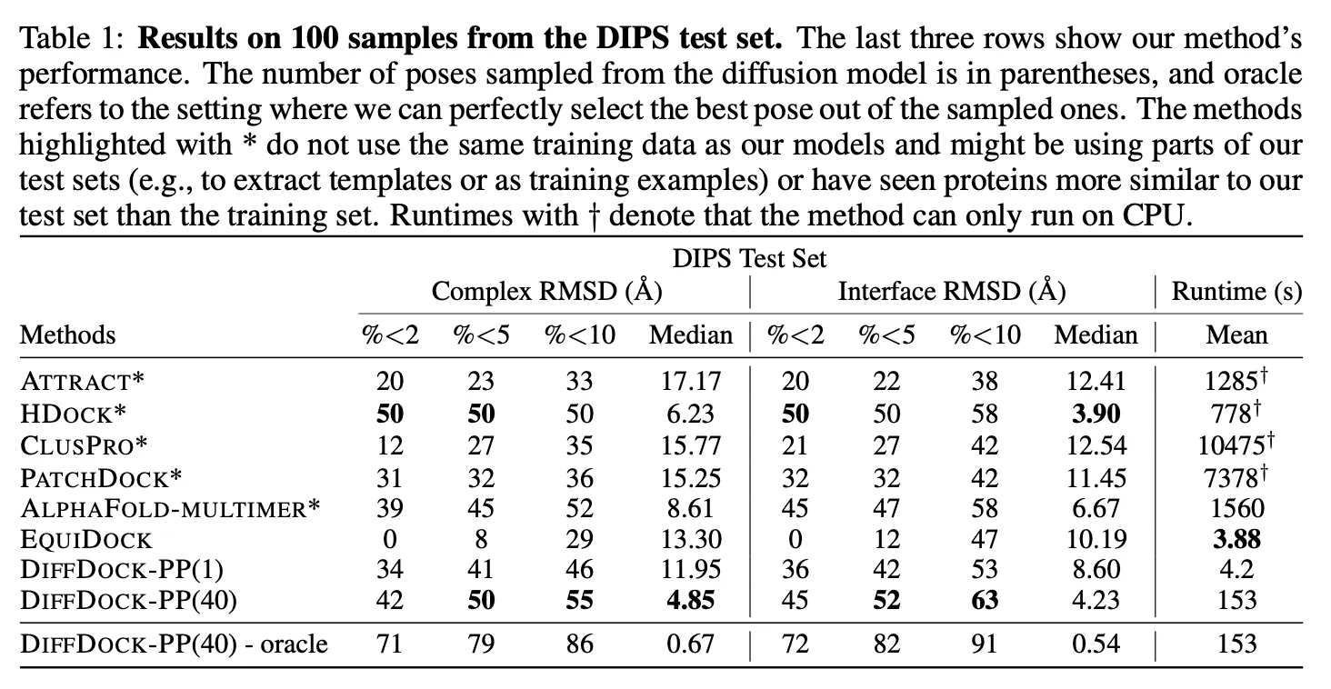
DiffDock-PP (40개 generation 후 best 뽑았을 때)는 C-RMSD median 기준 4.85 달성. C-RMSD와 I-RMSD 모두 높은 성능을 달성했다.

1개만 generation 했을 때도 괜찮은 성능을 보였다.

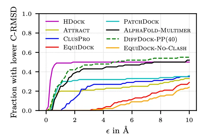
예측된 구조의 C-RMSD 누적 분포.

HDock이 5Å 미만인 것들이 많긴 한데, 5Å 이상으로는 DiffDock-PP가 그 비율이 더 높다.

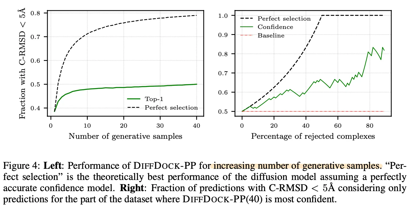
Confidence model의 성능을 보기 위한 그림.

Left: Top-1 (highest confidence score) vs Perfect selection (smallest C-RMSD 갖는 것. confidence score는 무시.) 비교. Confidence model이 잘 학습되었다면, RMSD 값이 낮은 것을 높은 confidence score로 예측했을텐데 top-1과 perfect selection 간의 gap이 꽤나 큰 것으로 보아 confidence model을 좀 더 잘 학습시킬 여지가 있어보인다.

Right: 특정 threshold의 confidence 이상인 것들만 남겼을 때, 즉, 상위 몇 % (x축)만 남겼을 때 C-RMSD 값 기준으로 5Å 으로 들어오는 것의 비율 (y축)이 얼마나 되는지 그려본 것이다. 역시 성능 개선의 여지가 좀 있어보인다.

6. Conclusion

DiffDock-PP는 DiffDock (protein-ligand docking)을 기반으로 하여 generative model로 protein-protein docking을 접근한 연구이다.

현존하는 deep learning 기반의 model 대비 높은 성능을 보였고, 현존하는 search 기반의 알고리즘들과도 맞먹는 수준의 성능을 보여줌과 동시에 빠른 속도도 보여주었다.

7. Major Takeaways

•

Protein-ligand docking에 접목했던 diffusion generative model이 protein-protein docking에도 유효하게 작동하는 것 같다.

•

Rotation, translation이 정의되는 manifold 상에서 diffusion을 수행한다.

•

Confidence model을 따로 학습해서 사용했다.